


Neural Networks Less Hard - Part 1
An introduction to neural networks that anyone can understand.

Goal: My goal for this tutorial is to teach you how neural networks (aka Deep Learning) work from basically nothing to a foundational understanding, including the underlying mathematics.
Assumptions: The only pre-requisites I assume is that you have a middle or early high-school level mathematics background, basically meaning you can comfortably solve for x in algebraic equations like 3x+5 = 11 and understand functions like f(x) = m*x + b and graph points on an X-Y plane. These tutorials do include some computer code (using Python), and while knowledge of at least basic programming will be helpful, it is not necessary as this multi-part series of posts are focused on the concepts rather than a concrete code implementation. I will teach you all the rest, including basic calculus and probability theory. The only catch is that this is long and moves slowly. But if you follow along, you will understand and be able to do Deep Learning by the end.
Motivation: There are many books, tutorials and resources that teach deep learning and neural networks, but most of them either assume way too much of the reader or only teach it superficially. Neural networks are actually quite simple fundamentally. Modern deep learning algorithms are complex but that’s only because they add a lot of fancy bells and whistles to a simple foundation.
Background: Neural networks are what power all the technology called artificial intelligence these days (such as ChatGPT and other large language models). The category of modern neural networks are often referred to as Deep Learning. Deep Learn algorithms (aka neural networks) can be used to predict what you’re going to type next in a text message, generate realistic images, drive cars, optimize energy usage in factories and many many other tasks all by learning from data; that’s what makes them so powerful.
Here is how neural networks are often first introduced and depicted in a tutorial (straight from wikipedia):
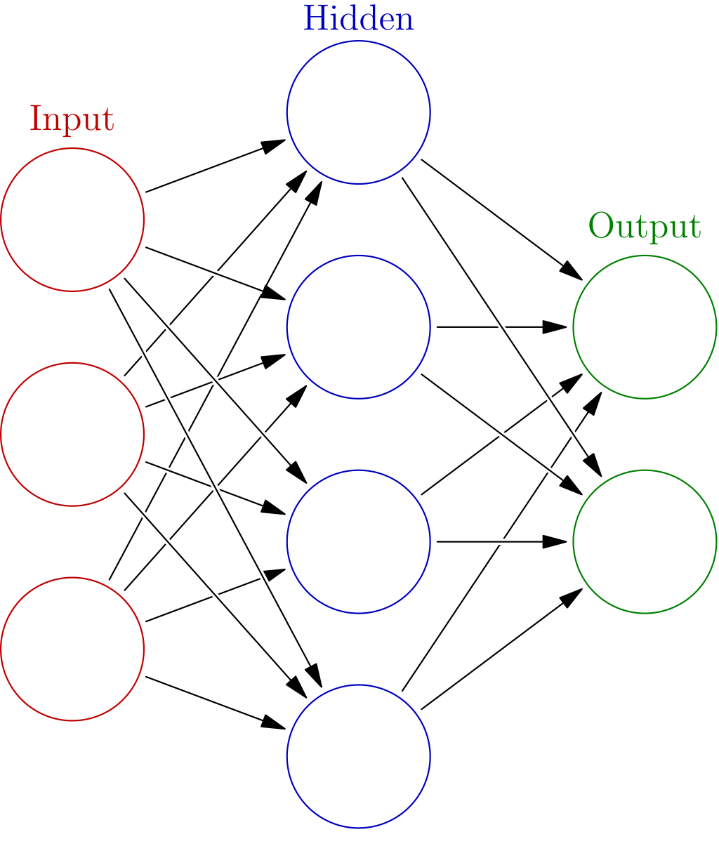
Neural networks are often introduced by referencing their relationship to biological neural networks, where you have “neurons” (or nodes) connecting and sending information to other neurons in different “layers” via their connection “weights.” The fact that modern neural networks have multiple layers in series is where the “deep” in Deep Learning comes from.
In more detail, some input data (in the form of some numbers) gets multiplied with weights (aka parameters), which then gets processed by neurons (aka nodes) that then return output number(s), that then goes through the same process.

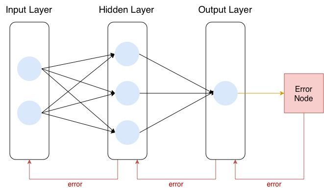
Training the neural network usually uses a procedure called backpropagation, which involves sending error signals back through the neural network graph to update the weights of the network. Often this is depicted as an “error unit” sending an error signal back to the output layer, which sends its own error signal back to the prior layer and so on.
That is not an inaccurate depiction, but it obfuscates how to actually implement a neural network in code, and if you don’t know how to implement a neural network in code, you don’t understand neural networks.
Let’s demystify.
A neural network (Deep Learning) is a nested function.
What is a nested function? A nested function, also called a compositional function, is a function that has other functions inside of it. It’s like if you have a box inside of a box inside of a box inside of a box, where each box is a function. Now, I want to make this as accessible as possible, so let’s backup and define what a function is.
Definition: A function is a rule that takes some input data and assigns it to or transforms it into a different form (the output data).
This is a fairly broad definition of a function. A function can therefore be as simple as a table like this:

The instructions for this function are just to find the input in this table and then the adjacent cell under the Output column is the output of this function. This is called a lookup table.
We could have defined a similar function using more operational instructions as opposed to a look up table. For example, we could have defined this function as: take each digit of the input number and flip it, so if a digit is a 0 then flip it 1 and if its a 1 then flip it to 0.
A function transforms individual instances, or elements or terms or values (all equivalent terms) from a particular input space or set or type (all equivalent terms in this context) into new values of a potentially different output type. For example, the input type of our first binary function using the lookup table is the type of binary numbers of length 2, because that is only what our lookup table shows, and the output type is the same. The input type of our second more operationally defined function is the type of all binary numbers of any length, since it flips the individual digits of a binary number.
A type can be thought of as a specification of a certain set of values that you want to define as a group. Another way to think of a type is as a constraint. Rather than letting a function consume any possible value (whether it be a number, or English characters, or something else) you define a type as a constraint on what is allowed for the function to ingest (input) or return (output).
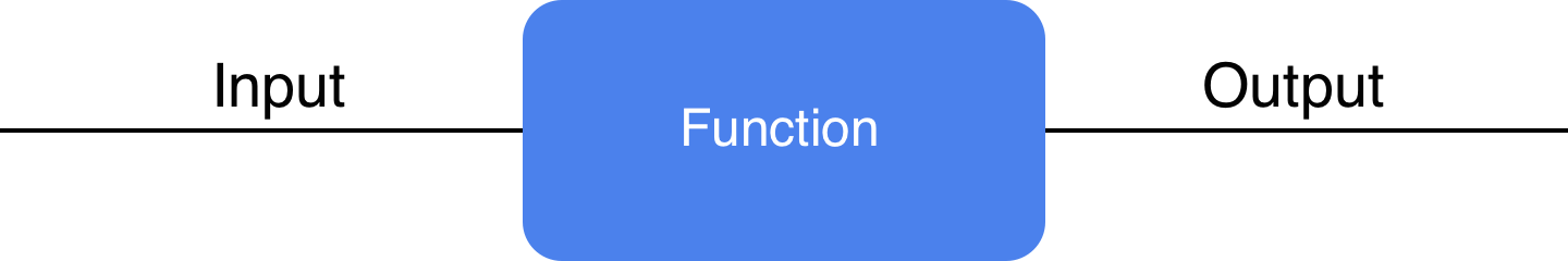
I like to think of functions like little machines where input material gets sent inside along a conveyor belt from the left and this input material gets transformed into some output material that then gets sent out on the right side on another conveyor belt. This lends itself to a nice graphical view of functions, which are called string diagrams because it looks like they have little strings going in and out, representing data going in and coming out:
I also like to annotate the input and output types
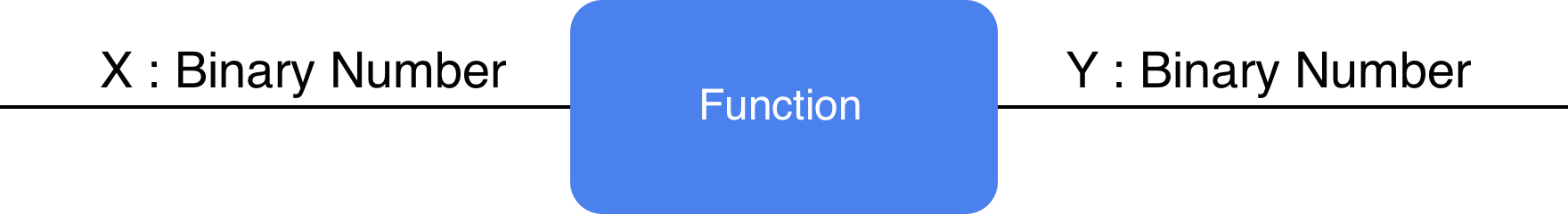
Okay, so now that we have a good idea of what a function is, let’s demystify a compositional function (aka nested function). A compositional function is just a function that is composed of multiple functions, and therefore can be decomposed into a set of separate functions that are applied in sequence. Let’s see this graphically.

Here I’ve defined two functions, Function 1 takes a binary number as an input and returns a new binary number as output, then it passes that value into Function 2, which transforms that binary number into some English letters like A, B, C, etcetera. I could keep these as just two separate functions, but if I package them together and give it a name, now we have a nested or compositional function.
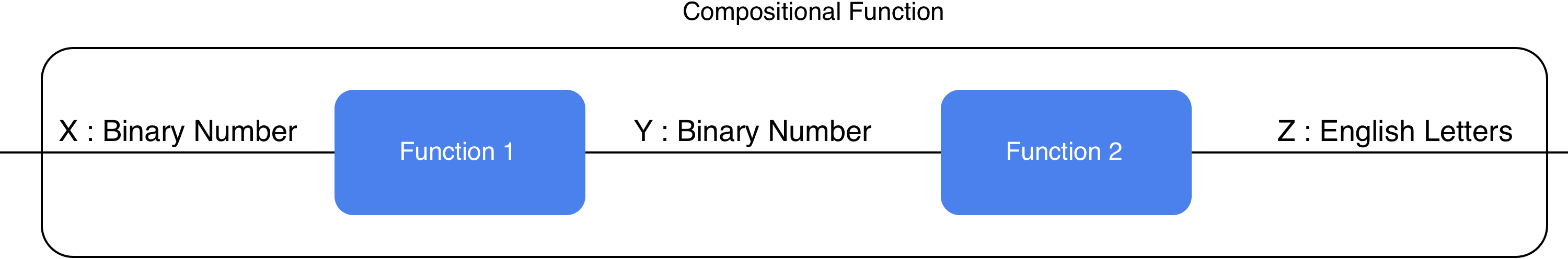
In typical mathematical and programming notation, you would call this function like so: function2(function1(X)). First you apply function1 to X, and then apply function2 to the result of that.
And that is the essence of deep learning. The “deep” in Deep Learning is just about these kinds of compositional (or nested or sequential) functions. That’s basically it. We will have to wait to understand the reason why deep learning (using compositional functions) is so powerful until later. Also, I’ve left out the details of what the composed functions actually do in a neural network at this point, but even that is not too complicated. Let’s keep going.
A neural network looks just like the figure above, except we often call each of those “inner” or composed or nested functions a layer (instead of Function 1 and Function 2), and each layer function takes a vector as an input and returns a new vector as an output instead of individual numbers.
A layer in a neural network is just a function that takes a vector and transforms it into a new vector.
Layer functions are the most basic unit in a neural network. Multiple related layers can be grouped together to form modules or blocks.
Layer functions transform the input vectors by 1) multiplying them with a matrix and 2) applying a non-linear activation function. Again, to make this as accessible as possible, I’m going to assume you have no idea what vectors or matrices are, and have no idea what a “non-linear function” means.
But let’s start with a concrete problem to solve and work our way to an understanding of these concepts. We will do this by studying a non-deep learning problem (i.e. it is only one “layer” deep).
Non-Deep (Shallow) Learning
Let’s say you are a climate scientist and you’ve collected some data about the global mean (average) temperature over the past several decades.
The global mean temperature for a particular time period is the average temperature of Earth’s surface over that time period. To calculate it, meteorologists and climate scientists collect temperature data from thousands of weather stations on land, from sea vessels, and from satellites measuring atmospheric and surface sea temperatures. They then combine these readings to estimate the average temperature of the entire surface of the planet.
Often, scientists calculate what is called the temperature anomaly, which is the difference in the global mean temperature for each year compared to the long-term average during some reference period. For example, if the average temperature for the years 1951-1980 was 14°C, and the global mean temperature for the year 1880 was 13.83°C (which is 0.17°C lower), then the temperature anomaly for 1880 would be -0.17 relative to that reference period. So the temperature anomaly is just how much the temperature deviates from some chosen reference value.
Here’s a plot of the global mean temperature anomaly over the past several decades:
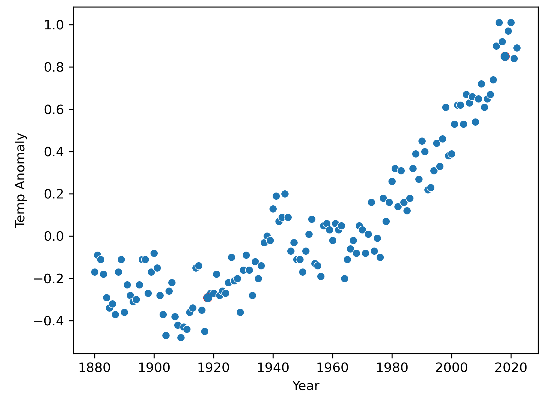
As you can see, there is a clear trend for the global mean temperatures to increase over time toward the present. If we want to predict what the temperature anomaly will be in the year 2040, we will need a model of the temperature anomaly as a function of time, and possibly other inputs.
A model in general is a compressed representation of something real, for example, a model rocket that a child may have is a literally compressed representation of a real rocket. As a model, it can be useful if you wanted to show someone who’s never seen a rocket before what it looks like, and you could use it as a prop to explain various functions of the rocket.
A model in the machine learning and artificial intelligence context is a compressed representation of 1) a process with inputs and outputs that we care about, or 2) of data generated by such a process.
Most useful compressed representations, i.e. models, in the machine learning context are inaccurate to some degree. That toy model rocket conveys a fair amount of truth about real rockets, but it can’t get to the moon. Likewise, machine learning models are meant to be useful but they aren’t likely to exactly capture all the details of the real process.
A compressed representation in machine learning is going to be a computational representation, meaning something we can represent on a computer or mathematically. This could be as simple as a table of data that captures the essence of a process. In fact, the data graphed in figure 3 could be called a model of the real, much more complex and highly detailed trend of say the daily or hourly temperature anomalies.
A process is essentially another way to say function, i.e. something that takes input material or data and produces output material or data. We’ve already learned how to graphically represent processes using string diagrams earlier. The underlying process that generates Earth’s global mean temperature is extraordinarily complex involving physical interactions from the tiniest scales to the largest scales on Earth, so any model we generate is going to be highly simplified. In fact, we can’t even collect all the data that represents the appropriate inputs to this process (which might involve knowing where all the clouds are among many other variables, for example). All we have is the temperature anomalies over time.
But, we can make an assumption that past predicts future, and we can model this process as a simple function of time like this:
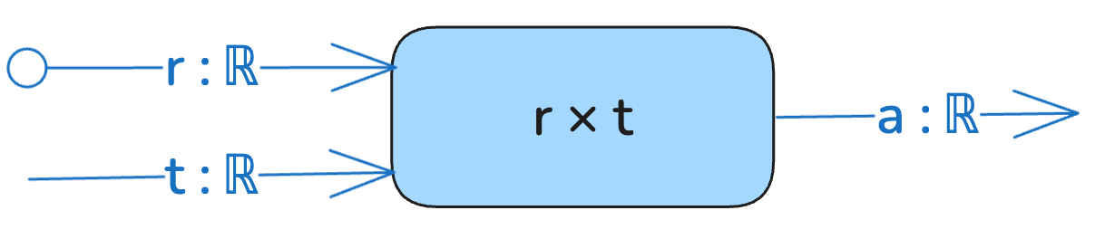
This is a function that constructs a linear model of the temperature anomaly data over time. A linear model is a model (i.e. a function that is a compressed representation of some data or process) that simply models the output as a rescaled version of the input. This string diagram takes a single input t for time, and it is of type ℝ, which is the symbol for real numbers. Real numbers are the term in mathematics essentially for arbitrary decimal numbers like 4.10219 or -100.0003. In a programming language, real numbers would correspond most closely to floating point numbers. Real numbers are the most common type of numbers we will see, but sometimes we will deal with binary numbers or integers (which are the whole numbers like …-3, -2, -1, 0, 1, 2, 3…).
Our linear model takes a time (in years) represented by the variable t and scales it by the parameter r to produce the output a, that is, our linear function (model) is just a(t) = r × t. A parameter is an input to the function or model that is fixed for some period of time, it does not freely vary like a variable such as t. I represent adjustable (also called trainable) parameters using the open circle at the end of the string. I represent fixed parameters using a solid circle at the end of the string (not yet depicted).
In this case, you can think of r like a simple conversion factor. Since t is in years, r would have the units °C/Years, such that the units cancel out to give us what we want, i.e.

That is, r tells us how many °C the temperature anomaly will increase (since r is positive) per year; it is a rate of change.
Our linear model defines a line, so we want to choose a value for r that makes the line model our data as best as possible. Let’s choose 2 points that seem to represent the data well at both ends.
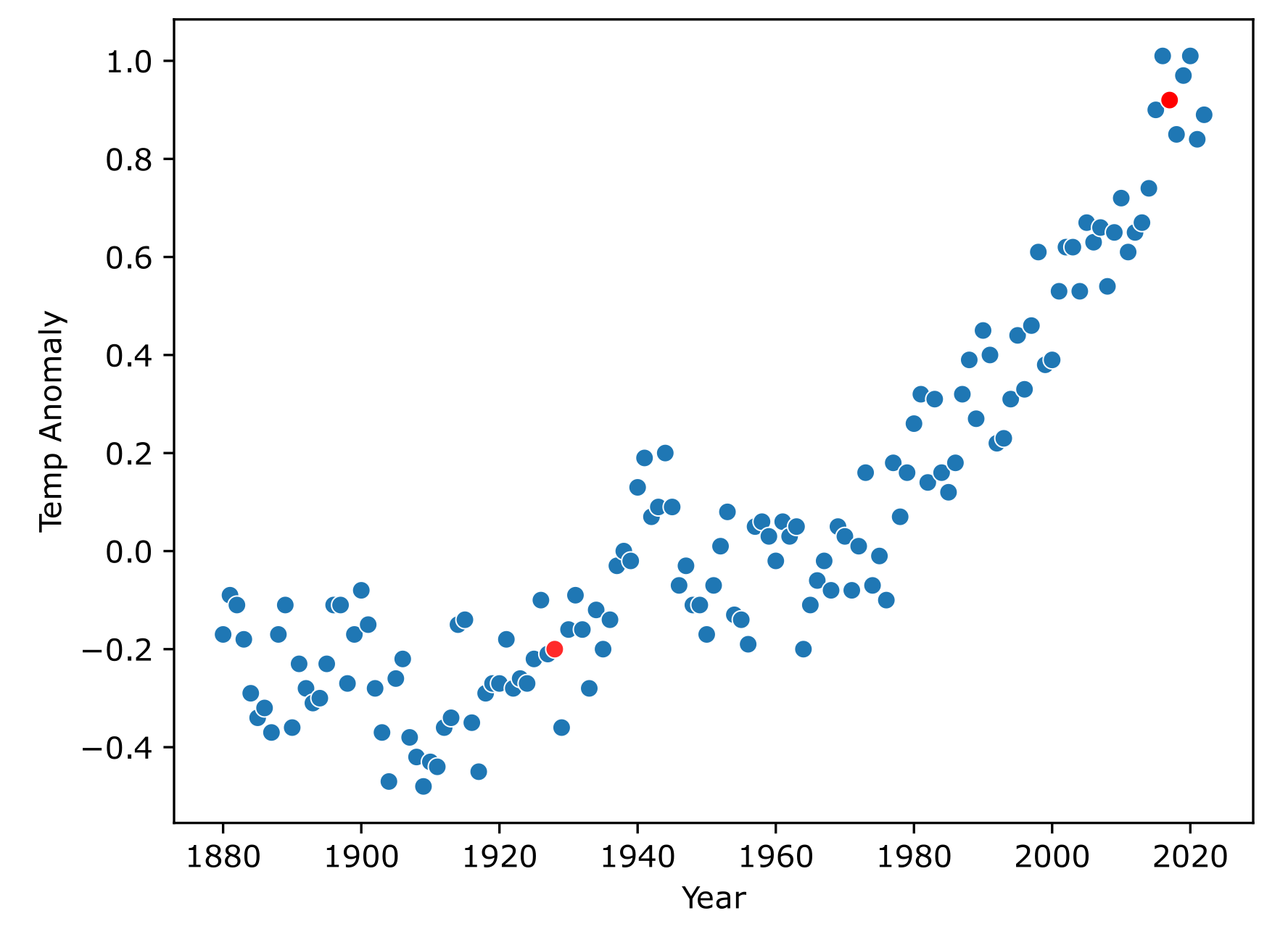
The points chosen were chosen just based on looking at this plot and selecting ones that appeared to represent the data near both ends. The point on the left, which we’ll call p₁, is at (x = 1918, y = -0.29) and the point on the right, which we’ll call p₂, is at (x = 2018, y = 0.85). Knowing these points, we can find the appropriate value for r.

We’ve figured out the slope of the line, r = 0.0114, which fully determines our linear model, and means that for every 1 year increase in time, the temperature anomaly increases by 0.0114°C. So since in this dataset the last value recorded is for year 2022, with a measured temperature anomaly of 0.89, then we can predict on the basis of our linear model that in the year 2023 the temperature anomaly should be around r + 0.89 = 0.0114 + 0.89 = 0.9014. The actual temperature anomaly for 2023 was 1.14 °C, so pretty close to what our linear model predicted.
But what if I want to predict the temperature anomaly for the year 2030? Well, if my last known value is (year = 2022, a = 0.89), then 2030 represents 8 years in the future, so I need to add r 8 times, hence, (year = 2030, a = 8 × r + 0.89 = 0.9812). Having to figure out the difference in years and then multiplying that by r is a little inconvenient, and this dataset will keep growing each year, so my last known value will change, meaning I have to change my calculation each time I want to predict out in the future. It would be better if I just had a function that takes in the year and spits out the predicted anomaly without reference to my last known data, like the string diagram I showed earlier.
We can do that, but we need to introduce an offset (also called, intercept, or bias in the machine learning context). See, as it stands now, knowing r only tells us by how much the temperature anomaly will increase per 1 year, so to predict into the future we have to pick a changing reference point to add to. In order to get a nice function we can just plug any year in and get what we want, we need to have a fixed reference year. Let’s pick one of the two points we used to define our line as our fixed reference point, let’s choose p₁ = (x = 1918, y = -0.29). It doesn’t matter which point we pick as long as it’s on our line.
Now we can make a new equation:
a = (y - 1918) × 0.114 - 0.29… which is of the more general form:

where y is any year you want to input, y_ref is the fixed reference year we choose, r is our conversion rate (slope), and a_ref is the temperature anomaly for the chosen y_ref reference year. Now we can do a little algebra; let’s first distribute the r.

Let’s substitute back in our values for r, y_ref, and a_ref.
a = 0.0114 × y - 0.0114 × 1918 + (-0.29)
This rearrangement allows us to separate out the terms involving the year y and the fixed reference year y_ref = 1918. Now, let’s combine the constants:
a = 0.0114 × y + (-0.0114 × 1918 - 0.29)
a = 0.0114 × y - 22.1552
Notice that the term -0.0114 × 1918 – 0.29 = -22.1552 becomes our offset (aka intercept or bias), often denoted with the symbol b. This is the value of a when y = 0, giving us the y-intercept of our linear equation. Thus, the function of our linear model is now in the same form as the grade-school equation for a line y = mx + b.
This new linear model with a fixed reference allows us to calculate the temperature anomaly a for any year y, using a fixed reference point in time y_ref = 1918 and its associated temperature anomaly a_ref = -0.29, alongside our previously calculated rate of change, r = 0.0114.
Now we can add the line to the graph:
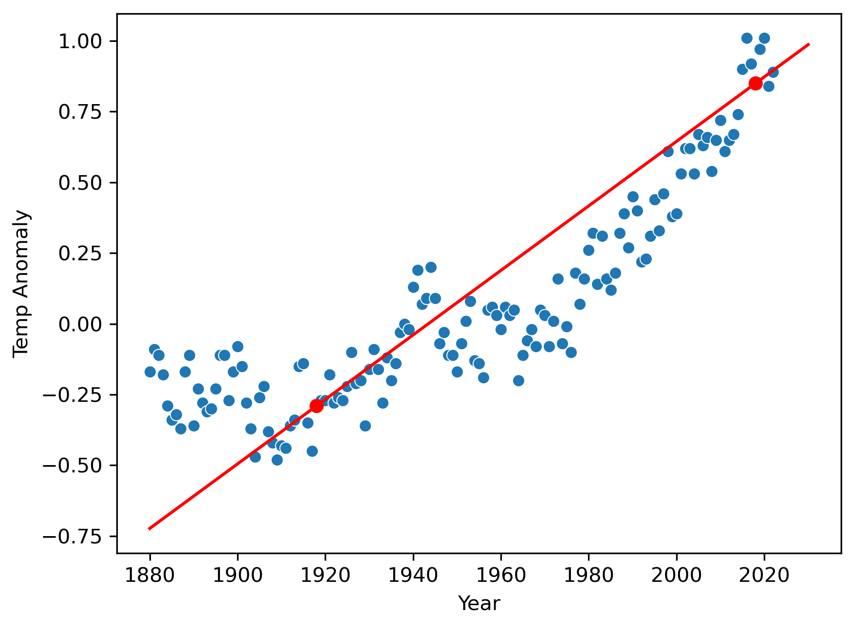
You can see our linear model doesn’t perfectly follow the data, mostly because the data is not perfectly linear, but it does a good enough job that we could probably use it to predict decent estimates of the temperature anomalies at least a few years into the future.
Summary
In this first part of the tutorial, we laid the foundation for understanding neural networks by exploring the fundamental concepts of functions and compositional (or nested) functions. We started with a simple definition of a function as a rule that transforms input data into output data, and then expanded to nested functions that combine multiple transformations in sequence. This progression helped us connect the idea of deep learning to these nested structures.
We also introduced the idea of modeling as a way to represent real-world processes in a simplified, computational form. Using a linear model to predict global temperature anomalies over time, we saw how to build and interpret a model with parameters like slope and intercept. This exercise sets the stage for understanding the role of layers in neural networks as mathematical transformations of input data. In part 2 we dive deeper into the necessary pre-requisites to fully understand neural networks.