


Neural Networks Less Hard - Part 2
An introduction to neural networks anyone can understand.

Recap of Part 1
In Part 1, we demystified the idea of neural networks as a series of nested (or compositional) functions. We broke down what a function is, how it transforms input data into output data, and how nested functions build on each other to form more complex transformations. We also introduced the concept of modeling, using a real-world example of predicting temperature anomalies with a simple linear model.
By the end of Part 1, you should have a solid grasp of how these foundational ideas—functions, nested functions, and models—relate to the "layers" in a neural network. Each layer can be thought of as a mathematical function that processes input data and outputs a new representation. In Part 2, we'll build on this understanding by diving into the mechanics of layers, vectors, matrices, and the non-linear activations that give neural networks their power.
The Space of Data and Models
Recall, our linear model from part 1 takes a single number (the year) and returns a single number (the predicted temperature anomaly), and it basically has a single trainable or adjustable parameter, r, although the offset (aka intercept or bias) is also considered a parameter.

We have been working with one-dimensional data. When we speak of dimensions of data, we are first implicitly recognizing that data live in a mathematical space. A space in the mathematical and machine learning sense is a way of recognizing the distinctions between different data and how they relate. For example, here’s just a part of the temperature anomaly data as a sequence of numbers:
[0.67, 0.74, 0.9 , 1.01, 0.92, 0.85, 0.97, 1.01, 0.84, 0.89]
Each number is the temperature anomaly for the years 2012-2022, in order. What can we say about the space that these data live in? Well, this space is composed of elements that are real numbers ℝ, which we introduced earlier. The elements of a space are like its atoms, it’s fundamental units (hence, elements being elemental). We also know that these elements have a temporal order, meaning we cannot just change the order, without disturbing the meaning of the data.
That leads me to perhaps the defining feature of a mathematical space:
A (mathematical) space is principally defined by what transformations (or moves) you can make in the space without fundamentally altering its meaning and structure.
A space’s structure is defined by how the data relate to each other. For example, if I were to change one data point from Celcius to Fahrenheit, then the meaning (i.e. semantics) of the space would not be changed (it is still a sequence of temperature anomalies over time), but the structure would change, since the difference in values would be quite large, and it would be difficult to work with.
On the other hand, if I were to convert all of the values into Fahrenheit, then the meaning and structure would be preserved. To convert into Fahrenheit, all we have to do is apply a specific mathematical transformation to each data point. The formula for converting a temperature from Celsius to Fahrenheit is F = C ⋅ 5/9 + 32, where F is the temperature in Fahrenheit and C is the temperature in Celsius (and the center symbol ⋅ is just another symbol for multiplication). By applying this formula to each value in our sequence, we can convert the entire dataset to Fahrenheit.
This transformation would change the numerical values but not the relationships between them: the way one temperature anomaly compares to another over time — remain consistent. The overall pattern, trends, and differences between consecutive years are preserved. In essence, the data tell the same story, but in a different ‘language’ or unit.
As I alluded to earlier, these data live in a one-dimensional space, and that is because we can identify each data point by a single address number. For example, here’s our data again, but I’ve given it a name T:
T = [0.67, 0.74, 0.9, 1.01, 0.92, 0.85, 0.97, 1.01, 0.84, 0.89]
Now I can say that the value 0.74 lives at address 2 from the left, and we can access the value by using this notation: T[2] = 0.74. We will see later that spaces with more than one dimension will require more numbers to identify and access the data.
Just to hammer this point in, let’s enumerate some of the features of this space:
The space can be uniformly scaled by a conversion factor (often called a scalar).
A single number can be added to or subtracted from each value, which essentially shifts the temperatures up or down without disturbing the semantics or relationship between points.
The space has a temporal order to it. We cannot move values around in the sequence arbitrarily.
The distance between points in the space is taken by their absolute difference.
We can course-grain the data by averaging over say 10 year blocks, which will not disturb the overall structure and semantics, it will just lower the resolution of the data.
Another way of thinking about a space is just like a type in a programming language with some constraints on what you can do with values of that type.
Let’s summarize what we’ve accomplished so far: We have built a linear model by choosing two representative points toward each end of the dataset and effectively drew a line through them to define our model. This linear model follows the trend of the data and thus could be used to predict future data. Is this a machine learning model? Arguably yes, it can be considered as a basic form of machine learning. Machine learning, at its core, is about creating models that can learn patterns from data and make predictions or decisions based on those patterns. Our linear model, although simple, does fit this description.
However, we as the human modeler were actively involved in “fitting” the model to our data. Usually when we think of machine learning models, there is an algorithm (aka procedure) that robotically figures out how to fit (aka train, or optimize) a particular model to the data, without us having to look at the data and do it ourselves. In this case, the training algorithm should automatically choose the conversion rate (slope) parameter r and the offset parameter b based on our data. There are a variety of training algorithms and we will learn how those work in more detail in another tutorial. In this tutorial, we will be manually training the models.
Vectors and Multidimensional Spaces
Our current linear model makes predictions about future temperature anomalies using only temperature information from the past. We can likely get better performance (i.e. more accurate predictions) from our model if it uses additional data to make its predictions. We know that greenhouse gasses like carbon dioxide CO2 in the atmosphere have an important impact on global average temperatures, so this seems like an important variable to include in our model.
Here’s what our new model looks like when it includes this additional input variable of average CO2 concentration measured in parts per million:
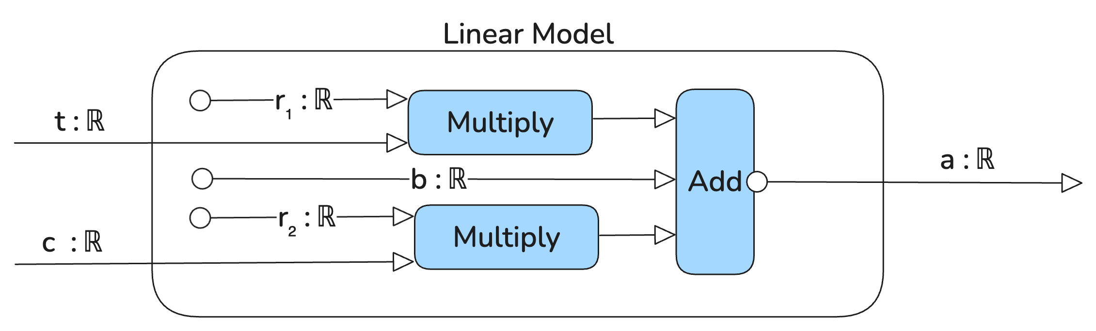
In mathematical notation this represents the function

with two inputs, time (year), and CO2 concentration in the atmosphere, r₁ and r₂ are scaling parameters and b is the offset parameter.
In this case, the diagram looks more complicated than the function in standard math notation, but in the future you’ll see how these kinds of diagrams can communicate complex neural networks succinctly.
Okay, now we have a function with two inputs, which we’ve name t (for time or year) and c for CO2. Since we cannot evaluate this function (i.e. run this program or process) until we have both inputs at the same time, it makes sense to package the two inputs into a pair (t, c) rather than treat them as completely separate inputs. The more general form of a pair is an n-tuple, where a 3-tuple is something like (a,b,c) where a,b,c are all some type of input variables, and a 4-tuple is something like (a,b,c,d), etcetera.
With some assumptions, these n-tuples form what what is called a vector space in mathematics, and thus, the n-tuples are also called vectors that live in the vector space. The study of vectors and vector spaces is the domain of Linear Algebra, one of the most useful fields in mathematics for machine learning. The known mathematical tools from Linear Algebra are critical to understanding and using neural networks.
Introduction to Linear Algebra
Recall, I previously introduced the concept of a mathematical space as a set of elements (or a type) and a set of allowable transformations (i.e. functions) on those elements (or values of the type) that preserve the structure and meaning (i.e. semantics) of the space. Well, a vector space is a space where the elements are called vectors and the allowable transformations between them are called linear transformations. Vector spaces, as mathematicians define them, are quite abstract and difficult to explain intuitively, but for machine learning purposes, we need not be that abstract.
Vectors as displacements
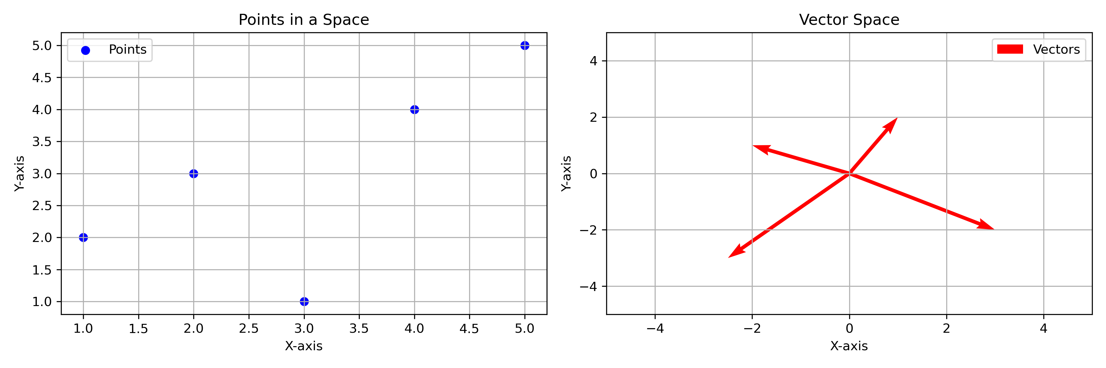
A vector space encapsulates the idea of displacement. Displacement is simply the amount and direction of change from one state to another, for example, traveling 2 hours is a displacement in time, or traveling 2 miles North is a displacement in space, or making a $500 deposit into your bank account is a displacement of money. Usually, displacements, unlike lengths or distances, have both a magnitude and an orientation (or direction). You can travel for +2 minutes, or you can rewind a video by 2 minutes, (i.e. the displacement being -2 minutes). You can go 2 miles north, south, east, west or any where in between. You can deposit money (e.g. +$500) or withdraw money (e.g. -$500). Vectors are displacements, and displacements are changes in state that usually have a size and an orientation.
In this sense vectors are conceptually different from “points” in a space. For example, 4:00 PM on a clock is a “point” in “time space.” It is a static reference point. But a vector like +2 hours can be added to the point 4 PM, moving us to the new point of 6 PM. Similarly, a specific location on a map is a point, and a vector might be “200 meters east,” such that we can add this vector to some point-like location and get a new location. Points in space do not inherently convey movement or change; they are static and absolute locations. It generally doesn’t make any sense to add static points in space, e.g. Tokyo + New York = ?, or 4 PM + 2 PM = ?.
Abstract vector spaces
Mathematically, vector spaces are defined as a set of elements, equivalently, a type with values (called vectors) such that you are allowed to add any two vectors and the sum will also be a vector in the set (or space or type), which is a property called closure. You are also allowed to scale up or down any vector by multiplying it by a number (called a scalar) and the result is also a vector in the same space, a property called scalar multiplication. There must also be a “zero vector” 𝟘 such that for any vector v in a vector space, 𝟘 + v = v, which is a property called additive identity. Thinking of vectors as actions, displacements or state changes, the zero vector is essentially the “do nothing” vector. Lastly, each vector v in our vector space must have an additive inverse -v, such that v + (-v) = 𝟘. Additive inverses are essentially “undo” or “reverse” vectors.
This is a very general and abstract definition and thus many things can qualify as a vector space. In fact, (real) numbers themselves qualify as a vector space, since you can add any two numbers and get another number and you can also multiply a number and you still get a number. And these numbers could semantically represent whatever you want, for example money in a bank account that can be added or withdrawn or scaled up (e.g. due to interest).
Families of functions can form a vector space, such as the set of polynomials f₁(x) = x² or f₂(x) = 2x³ + x because these kinds of functions can be added (e.g. f₁ + f₂ = 2x³ + x² + x), scaled (e.g. 4 * f₁(x) = 4 * x²), have additive inverses (e.g. f₁ + -x² = 0) and additive identity functions (e.g. if f₀(x) = 0, then f₀ + f₁ = f₁). Note how in this case each vector is in a sense an infinite object, since these functions are defined over all real numbers from negative to positive infinity.
Most of the time in the machine learning context, we are dealing with vectors that are not that abstract and are just some numbers in a list, in which case we can think of these less abstract vectors as objects with direction and magnitude as opposed to points in space, which have a position (see figure 12).
Vectors in vector spaces can sometimes (depending on the context) be thought of as having multiple “components,” for example, like ingredients in a recipe. Consider the “space” of ingredients of cucumbers, sugar, sesame oil, and soy sauce. Simply mixing these ingredients, in the proper proportions, can make a delicious and simple cucumber salad. Let’s represent these ingredients symbolically, such that C = cucumbers, S = sugar, O = (sesame) oil, and Y = soy sauce. Then we can say a particular recipe for this salad is the combination a · C + b · O + c · Y + d · S, where a, b, c, d are numbers representing the amounts of each ingredient, e.g. number of cucumbers and tablespoons for the rest.
A specific recipe might be represented as 2C + 1O + 2Y + 1S, signifying a recipe with 2 cucumbers, 1 tablespoon of sesame oil, 2 tablespoons of soy sauce, and 1 tablespoon of sugar (I removed the multiplication · symbol for brevity, i.e. 2C = 2 · C). This is a vector in our vector space of cucumber salad recipes. We can more compactly represent this vector as simply an ordered list of numbers: [2, 1, 2, 1] where each position represents the amount of cucumbers, oil, soy sauce, and sugar, respectively.
This space of ordered lists (aka 4-tuples) of numbers representing recipes constitutes a valid vector space because:
Closure: The sum of any two recipe vectors (4-tuples) is another valid recipe vector in the space. For example, adding
[2, 1, 2, 1](one recipe) to another, like[1, 0.5, 1, 0.5], results in[3, 1.5, 3, 1.5], which is still a valid recipe representation in this space.Scalar Multiplication: Multiplying a recipe vector by a scalar (a number) scales the quantities of each ingredient and results in another valid recipe vector. For instance, 2 · [2, 1, 2, 1] = [4, 2, 4, 2]. This is useful if we want to scale our serving size up or down.
Additive Identity and Inverse: We have a zero vector 𝟘, namely, [0, 0, 0, 0](meaning no ingredients; do nothing), which acts as the additive identity. And each vector has an additive inverse, allowing for ‘undoing’ a recipe, for example the vector [-1, 0, 0, 0] corresponds to removing 1 cucumber. Remember, vectors are displacements so these vector recipes actually represent actions (not fixed states like points), e.g. the vector [2, 1, 2, 1] means we add 2 cucumbers, 1 tablespoon of sesame oil, 2 tablespoons of soy sauce, and 1 tablespoon of sugar to our (presumably empty) bowl. Each component in the vector represents an action to be taken with a specific ingredient.
Each vector in this space represents a valid recipe, but not all of them are going to be tasty.
But notice, in order to set this up as a usable recipe, we had to choose specific units (e.g. tablespoons) to use for each ingredient. These choices represent a chosen basis for our vector space. In this recipe vector space, the basis vectors are the standard units (like one cucumber, one tablespoon of oil, etc.). Every possible cucumber salad recipe (vector) in this vector space can be described using a combination of our chosen basis vectors.
More mathematically, our basis vectors can be represented like this [1,0,0,0], [0,1,0,0], [0,0,1,0], [0,0,0,1]. Each basis vector represents a unit quantity of one ingredient while having zero quantities of the others. For example, [1,0,0,0] represents adding one whole cucumber and no other ingredients. Similarly, [0,1,0,0] represents adding one tablespoon of oil without adding any cucumbers, soy sauce, or sugar. Any valid salad recipe (vector) can be constructed by adding these basis vectors and multiplying them by scalars. For example, our first recipe of [2, 1, 2, 1] can be seen as adding two units of the cucumber basis vector, one unit of the oil basis vector, two units of the soy sauce basis vector, and one unit of the sugar basis vector. In other words, it’s like 2 ⋅ [1,0,0,0] + 1 ⋅ [0,1,0,0] + 2 ⋅ [0,0,1,0] + 1 ⋅ [0,0,0,1]. This demonstrates how any recipe in this vector space can be constructed using linear combinations of these basis vectors.
A linear combination of vectors is simply creating a new vector by adding and scaling two or more other vectors. For example, let’s say we have two vectors named A and B, then we can linearly combine them to get a new vector C = a ⋅ A + b ⋅ B, where a, b are scalars (numbers).
This leads naturally into a discussion of what exactly linear means in this context.
Linear versus Non-Linear
We touched on the idea of something being linear when we introduced linear models earlier. But the idea of linearity is quite deep and interesting. Generally, we use the term linear to describe a function (transformation). You might think a linear function is one that defines a line if we graph it, and that is true to an extant, but we want a notion of linearity that can work for functions in 3-dimensions, 4-dimensions, and beyond.
Let’s start with the mathematician’s definition of a linear function. Recall that a vector space is basically defined as a type where we have an add operation and a scalar multiplication operation, and nothing else. Well, a linear function is a function that preserves these two operations. Preservation, in this context, means that if you have a function that is linear, let’s call it f, and operations of + and ⋅ (multiplication), then you get the same result whether you use + and ⋅ first and then apply the function f or if you apply the function f first and then use + and ⋅.
In mathematical terms, this means that a linear function f satisfies the following equalities, given two arbitrary vectors we’ll call u and v, and some scalar (number) called a.
f(u + v) = f(u) + f(v)
f(a ⋅ u) = a ⋅ f(u)
In other words, if we denote the + and ⋅ operations in our vector space as functions and just call them say t where t could mean either + or ⋅, then if a function f is linear and we have an arbitrary vector u:f(t(u)) = t(f(u)).
For example, the function f(x) = 2 ⋅ x is linear because
f(2 + 3) = 10 = f(2) + f(3) = 4 + 6 = 10.
Notice, however, that f(x) = 2 ⋅ x + 1 is actually not linear under this definition, despite it looking like a line when we graph this function, since
f(2 + 3) = 11 ≠ f(2) + f(3) = 5 + 7 = 12
So if both f(x) = 2 ⋅ x and f(x) = 2 ⋅ x + 1 look like straight lines when we graph them, why is only the former considered linear (in the context of linear algebra)? Well, because vector spaces capture the idea of a kind of conservation principle where you can’t get more out of a process than you put in.
Let’s pretend these simple functions are some sort of manufacturing processes that convert units of apples into units of applesauce. Our function f is now some process take takes in some number of apples and turns them into some amount of applesauce.

This looks very reasonable. You put in one apple and you get 2 units of applesauce (I leave the units unspecified here, maybe they’re cups or tablespoons or milliliters, it doesn’t matter). Also reasonable is the case if you put in 0 apples, you get 0 units of applesauce.
Now things get weird when we try our other linear-when-graphed-but-not-linear function:

If we put in 1 apple, we get 3 units of applesauce, more than the other function. Maybe this function is a more efficient way of producing applesauce, that’s certainly possible. But things get unreasonable when we put in 0. If we put in 0 apples, we will still get out 1 unit of applesauce. But how, where did this applesauce come from with no input apples? This process is apparently capable of producing applesauce out of nothing. That is what is non-linear about it. Linear functions don’t create stuff from nothing, 0 gets mapped to 0.
Let’s analyze another example function, say f(x) = x⋅ x, aka, f(x) = x². In terms of applesauce production, it could look like this:

If we put in 0 apples, we get 0 units of applesauce, so far so good. If we put in 1 apple, we get 1 unit of applesauce, if we put in 2 apples, we get 4 units of applesauce. Well if this was a linear applesauce maker, then if we put in 1 + 2 = 3 apples, we should get 1 + 4 = 5 units of applesauce. But we don’t, 3 apples in gets us 9 units of applesauce out.
Or more mathematically, f(1 + 2) = f(3) = 3² = 9 ≠ f(1) + f(2) = 1² + 2² = 1 + 4 = 5. So this function does not preserve the vector space operations, so that is why it is not linear.
Overall, we care about vector spaces because they nicely capture types of things that can be added and scaled, and we care about linear functions (transformations) because they transform one vector space into another vector space by preserving the vector space operations.
Linear Transformations as Matrices
Linear Algebra is about vector spaces and linear transformations between vector spaces. Linear transformations are often represented as matrices.
A matrix is often introduced as a grid of numbers, like this:

A matrix in the mathematical / programming context is just a rectangular grid of values of some type (generally numbers). Matrices can be used in two different ways: 1) as a linear transformation and 2) as a data table. In machine learning, we will use both types of matrices, but for now, we will focus on matrices as linear transformations.
Recall, our recipe vector space from earlier had 4 ingredients denoted C (cucumbers), O (sesame oil), Y (soy sauce) and S (sugar). We decided that the units for C is number of cucumbers and the rest are measured in tablespoons. Let’s consider a set of linear functions on this recipe vector space that converts the measuring units into a different set of units. We’ll write some functions that convert everything into grams. We’ll need 4 functions, one for each ingredient.

Note: I’ve used this new notation ↦ to define these functions without giving them names (just for convenience), called anonymous functions (also called lambda functions).
Now we can take any vector from the original recipe vector space, such as (3,3,3,1) representing 3 cucumbers, 3 tablespoons of sesame oil, 3 tablespoons of soy sauce and 1 tablespoon of sugar, and convert it into a new vector space where all the ingredients are represented in terms of grams.

So our new vector is (900,36,45,12). This vector represents the same recipe, just in a new unit vector space.
Each of the conversion functions were linear functions and thus the overall transformation is linear as well. Notice each of these linear conversion functions has a single conversion factor number; we can package these up into a matrix. Here’s what the matrix representation looks like:

There are a bunch of zeros because the linear functions we made are not interdependent or interacting with each other. Each conversion function operates independently on its respective ingredient, without influencing the quantities of the other ingredients. The zeros in the matrix represent this lack of interaction or cross-dependency between different ingredients in the recipe. In other words, changing the amount of one ingredient (like cucumbers) does not affect how the amounts of the other ingredients (like sesame oil, soy sauce, sugar) are converted into grams.
If there were interactions, we could have made a linear function like this:

In this case, we have a function that returns a new number of cucumbers based on not just the current number of cucumbers but also the amount of the other ingredients.
This might represent a situation in which the recipe’s balance or taste profile is adjusted according to the quantities of the other ingredients. For instance,
m₁could still be the direct conversion factor for cucumbers, but…m₂could represent how the amount of sesame oil influences the need for cucumbers (perhaps more oil reduces the need for cucumbers).m₃might show how soy sauce affects cucumber quantity (maybe more sauce requires more cucumbers to balance).m₄ could indicate a relationship between sugar and cucumbers (like more sugar balancing out the freshness of more cucumbers).
Some of these m parameters could be set to 0 if there is no interaction.
This reflects a more complex and interdependent relationship among ingredients than what is captured by simple unit conversions.
We could do the same for all the other ingredients, and then each ingredient would be converted into a new number by a linear combination (we learned about this earlier) of all the ingredients. Then for each of the 4 ingredients we’d have a linear function each with 4 scaling factors (also called coefficients), for a total of 4 × 4 = 16 coefficients. And recall, our matrix earlier had 4 rows and 4 columns.
To show how to use matrices, let’s first consider a simpler example.

This is a simple 2 x 2 matrix with entries labeled a, b, c, and d (representing some numbers). This matrix corresponds to two linear functions that transform a vector X with components x₁ and x₂, i.e. X = [x₁, x₂]:
f₁(x₁, x₂) = y₁ = a ⋅ x₁ + b ⋅ x₂
f₂(x₁, x₂) = y₂ = c ⋅ x₁ + d ⋅ x₂
As a reminder, these functions are linear because each input (i.e. x₁ and x₂) is only scaled and added to a number, and hence preserves the vector space operations of adding and multiplying.
Each one of these linear functions takes our input vector X = [x₁, x₂] and produces a new component of an output vector we could call Y = [y₁, y₂]. Each linear function multiplies the input vector components with 2 numbers (aka coefficients, parameters, scalars) and then adds them together. By packaging these coefficients into the matrix we can define a recipe for how to use this matrix to achieve the same effect as using these 2 linear functions, namely, we define a procedure for how to multiply a matrix with a vector to get a new vector.

To make this easier, let me first introduce the notion of the inner product or dot product of two vectors a and b is denoted a⋅b (note this is the same symbol for multiplication of numbers we’ve been using, but in this case these are vectors not just numbers), and is defined like this:

The greek upper case letter sigma ( Σ ) is the common mathematical notation for adding (summing). It is basically a for-loop where we add the corresponding components of two lists of numbers.
So, if you know some Python, here’s how you would implement the dot product as a function that takes 2 vectors (represented as lists of numbers for this example):
from typing import List

def dot_product(vector1: List[float], vector2: List[float]) -> float:
    """
    Calculate the dot product of two vectors.

    Parameters:
    vector1 (List[float]): The first vector.
    vector2 (List[float]): The second vector.

    Returns:
    float: The dot product of the two vectors.

    Raises:
    ValueError: If the vectors are not the same length.
    """
    if len(vector1) != len(vector2):
        raise ValueError("Both vectors must be of the same length.")

    product = 0
    for a, b in zip(vector1, vector2):
        product += a * b
    return product
Now that we’ve defined the dot product, matrix-vector multiplication can be explained as taking each row of the matrix M and then taking its dot product with the vector. So for each row of the matrix we will get a new number. For a 2 × 2 matrix like M above, we have 2 rows so we have 2 dot products yielding 2 new numbers, which form the components of a new vector.
Knowing this, we can write M(X) in a different way:M(X) = yᵢ = Mᵢ ⋅ X
The vector that results from multiplying the matrix M with vector X is arbitrarily called Y but each of the two components is labeled y₁ and y₂ or yᵢ more generally, where the subscript i is just some indexing number.
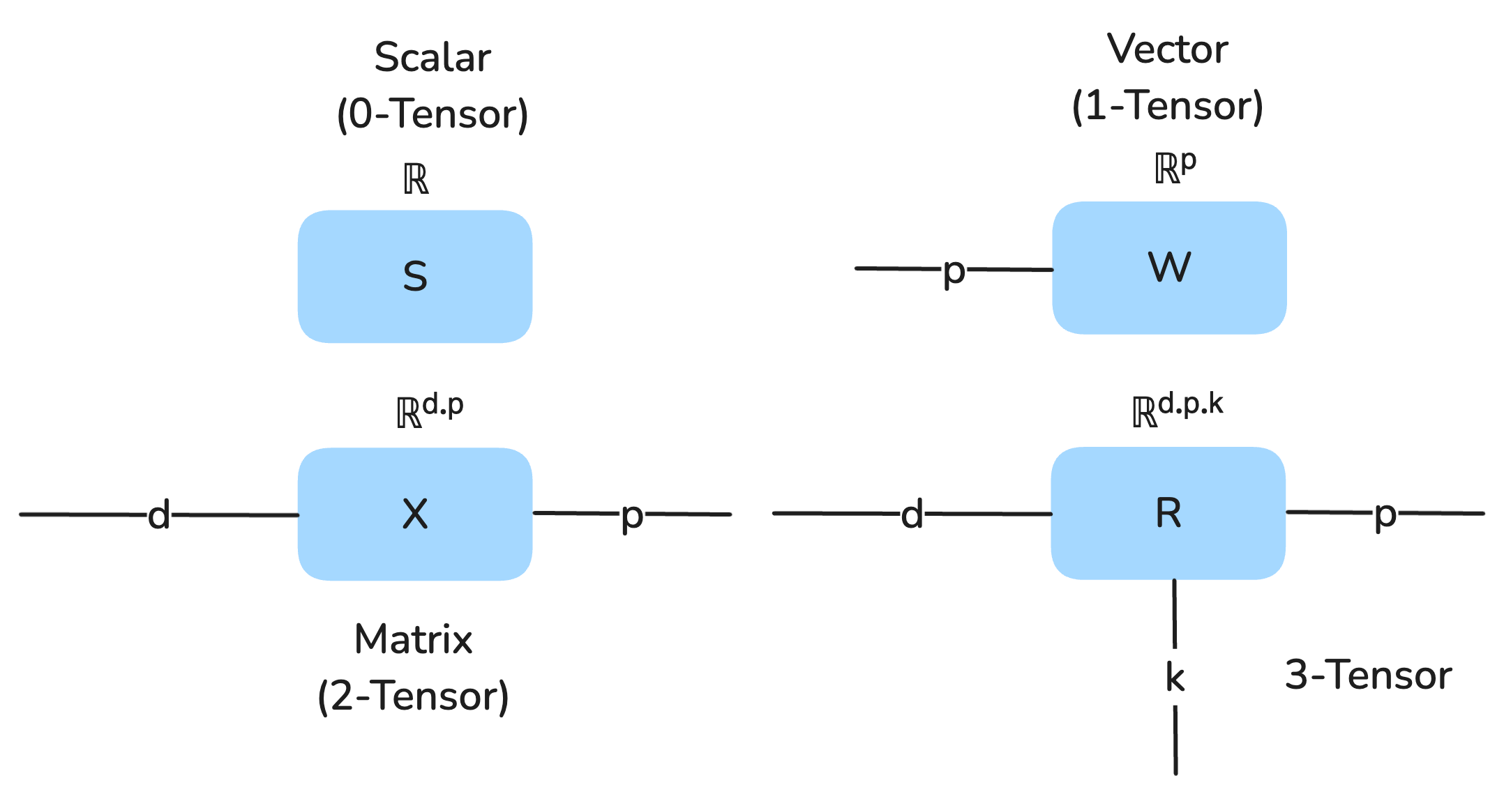
We call this notation indexing, which is a kind of addressing mechanism for vectors and matrices. A vector will have a single index which can take on values as long as the vector is. A matrix will have two indices since each value in the matrix has a corresponding row and column. There are also linear algebra types “beyond” matrices that have 3 or more indices (e.g. rows, columns, 3-D depth…) and we more generally refer to all of these as tensors. A 0-tensor is a single number (aka scalar), a 1-tensor is a vector, a 2-tensor is a matrix, and so on. The leading number indicates how many indices the tensor has.
So we can index (address) each row of the matrix M by giving it an index Mᵢ, where ᵢ can be any number as many rows as the matrix has, which is 2 in this case. So M₁ refers to the first row of the matrix. Thus each component yᵢ is computed by taking the dot product between the corresponding row Mᵢ with the full 2-element vector X.
To be concrete, given a 2 × 2 matrix M with some arbitrary numbers:
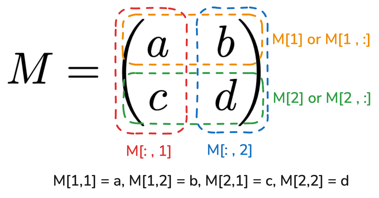
In mathematical notation and most programming languages, you can reference the elements of subslices of a matrix (or a tensor more generally) by specifying indices. For every N dimensions of a n-tensor, there will be N indices needed to reference a single element. In figure 13 the orange box highlights the first row of the matrix, and in many programming languages, you access this first row with a notation like M[1] or M[1,:]. In the case of M[1,:] you’re saying that you want row 1 and all the columns (denoted by the colon :), and this returns a vector that is the first row. In contrast, if you want a single element from this matrix with 4 elements total, you need to specify its specific row and column, e.g. M[1,2] references the element b.
Tensors are hierarchical in the sense that a 0-tensor is just a single number (a scalar), and a 1-tensor is a vector (e.g. a one-dimensional list of 0-tensors), and 2-tensor is a matrix, which is a collection of 1-tensors, and so on. So when you only specify a partial address, you get a lower dimensional tensor.
We can visualize scalars, vectors, matrices and tensors in higher dimensions as string diagrams.
Summary
Linear algebra is about linear transformations (functions) and the parameters of these linear transformations can be neatly packaged into rectangular grids called matrices, which themselves can become representative of the linear transformation by multiplying a matrix with a vector using the dot product. We need to grasp these basic linear algebra concepts to fully understand deep learning. Linear algebra is probably the most important ingredient in all of machine learning. We will keep building on these foundations in part 3.