


Neural Networks Less Hard - Part 3
An introduction to neural networks anyone can understand.

Recap of Part 2
In Part 2, we introduced linear algebra, the core mathematics behind neural networks, focusing on spaces, vectors, and linear transformations. We learned how data lives in mathematical spaces, where each data point can be represented as a vector. These vectors can be manipulated using linear transformations, which are neatly packaged into matrices. By working through examples like recipes and temperature anomalies, we saw how these transformations help us model complex relationships in data.
Using Vectors and Matrices in Machine Learning
We have barely scratched the surface on linear algebra, but we now know enough to use matrices and vectors to understand simple learning models, and later deep neural networks.
Let’s get back to our global temperature anomaly data and linear model:
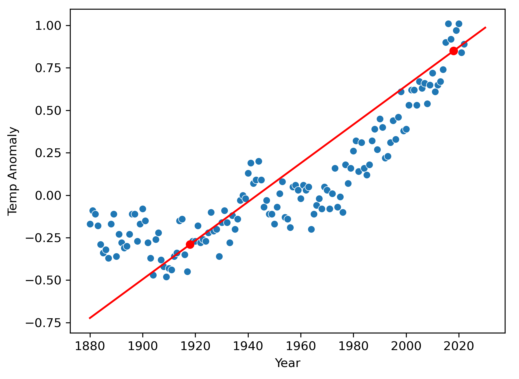
We earlier talked about extending this model to include two inputs, the year and the CO₂ concentration for that year, to be able to better predict the temperature anomalies. Here’s a plot of both of those data together:
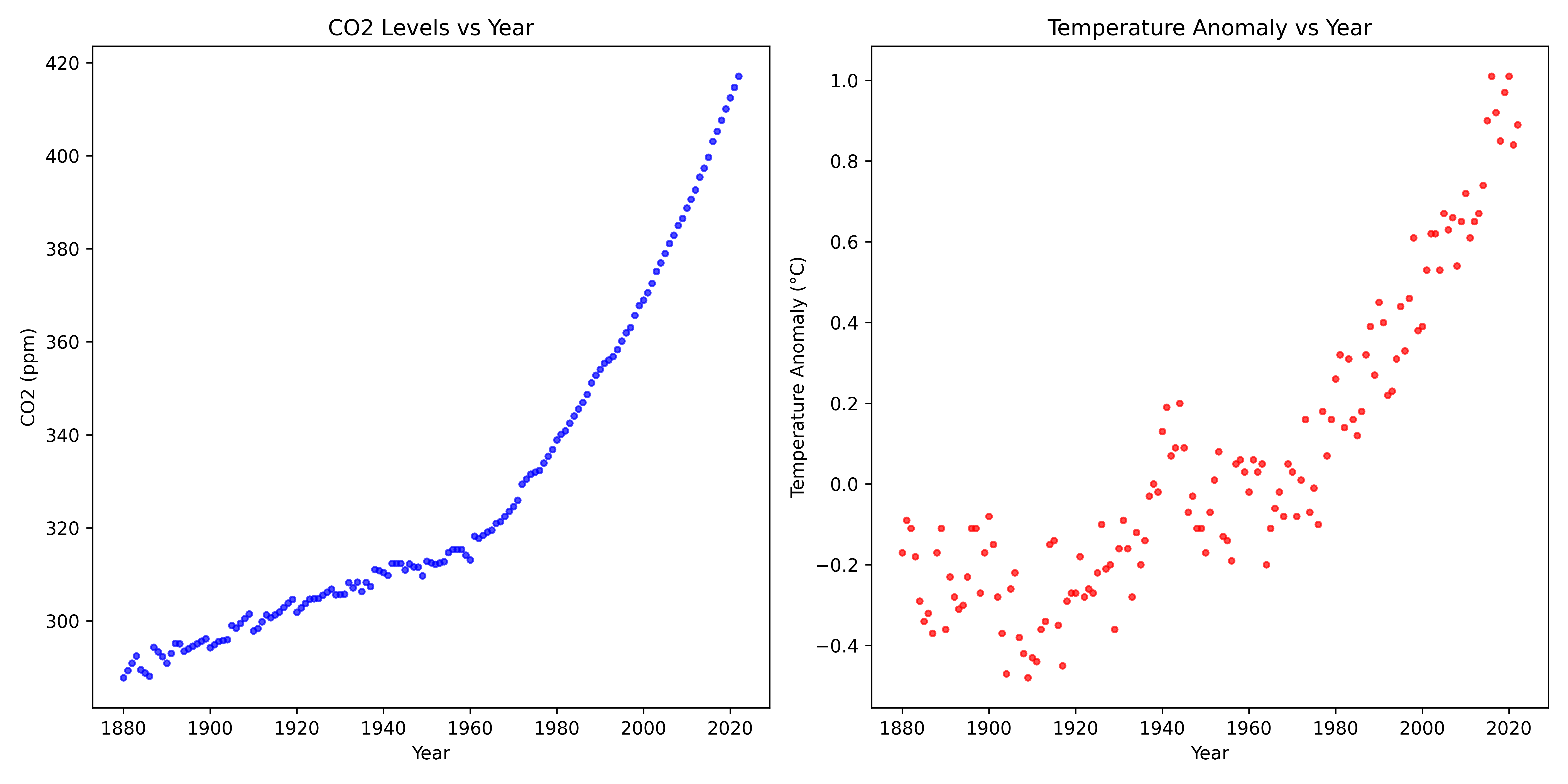
Annual CO₂ concentration seems to track the temperature anomaly pretty well over this time period, and given that we know CO₂ concentration has a causal role in determining global average temperature, including this variable in our model would likely significantly improve our ability to predict future.
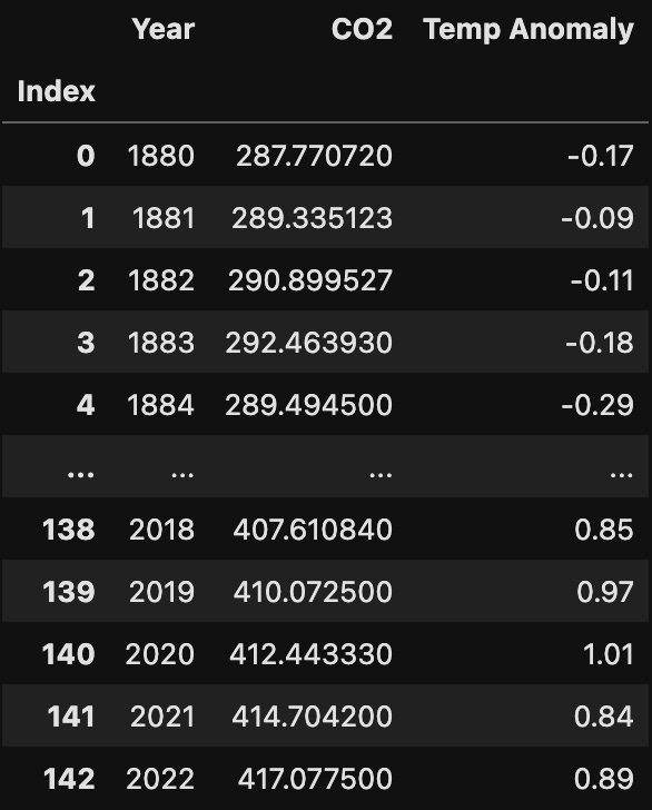
Here’s some of the raw data in table form:
Recall, this was the string diagram for our 2-variable model from earlier:
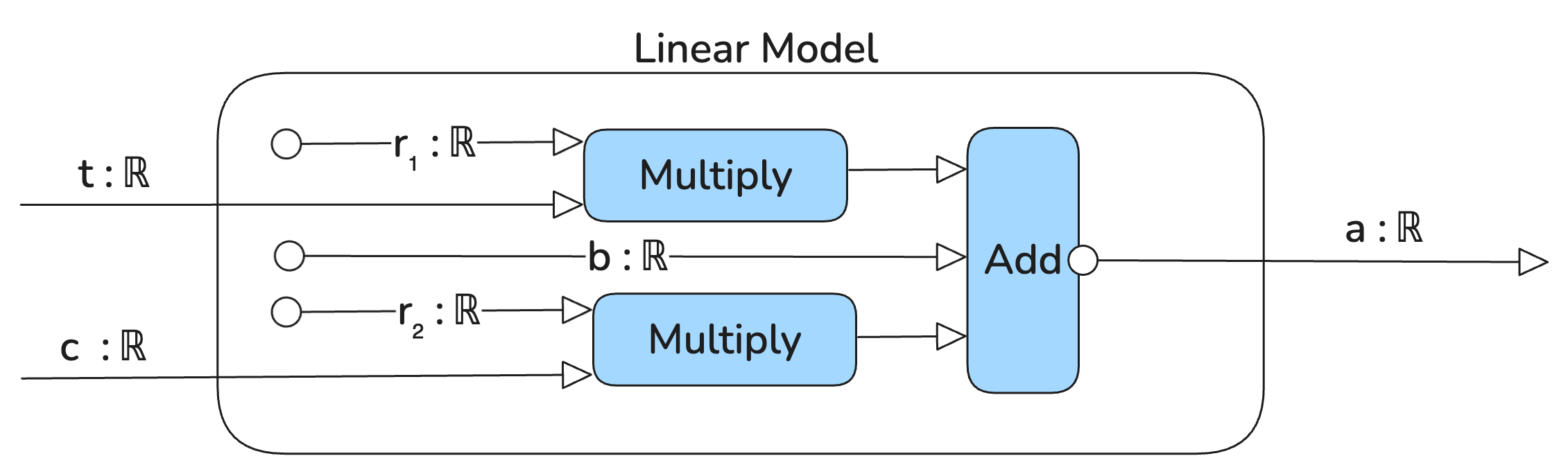
This corresponds to the mathematical expression:

But notice that this model cannot correspond to a simple line. We cannot just pick 2 representative points in each set of data (CO2 and temperature anomalies) and draw 2 different lines, because that would only allow us to predict CO₂ from CO₂ and temperature anomaly from temperature anomaly. We want to predict future temperature anomalies from past temperature anomalies and past or present CO₂ concentrations. That is why the model is a function of time (year) and CO₂ , so we can ask the model what the temperature anomaly will be for year 2050 if the CO₂ is say 400 ppm. To visualize this, we have to plot in 3-dimensions for the 3 variables (year, CO₂ and temperature anomaly).
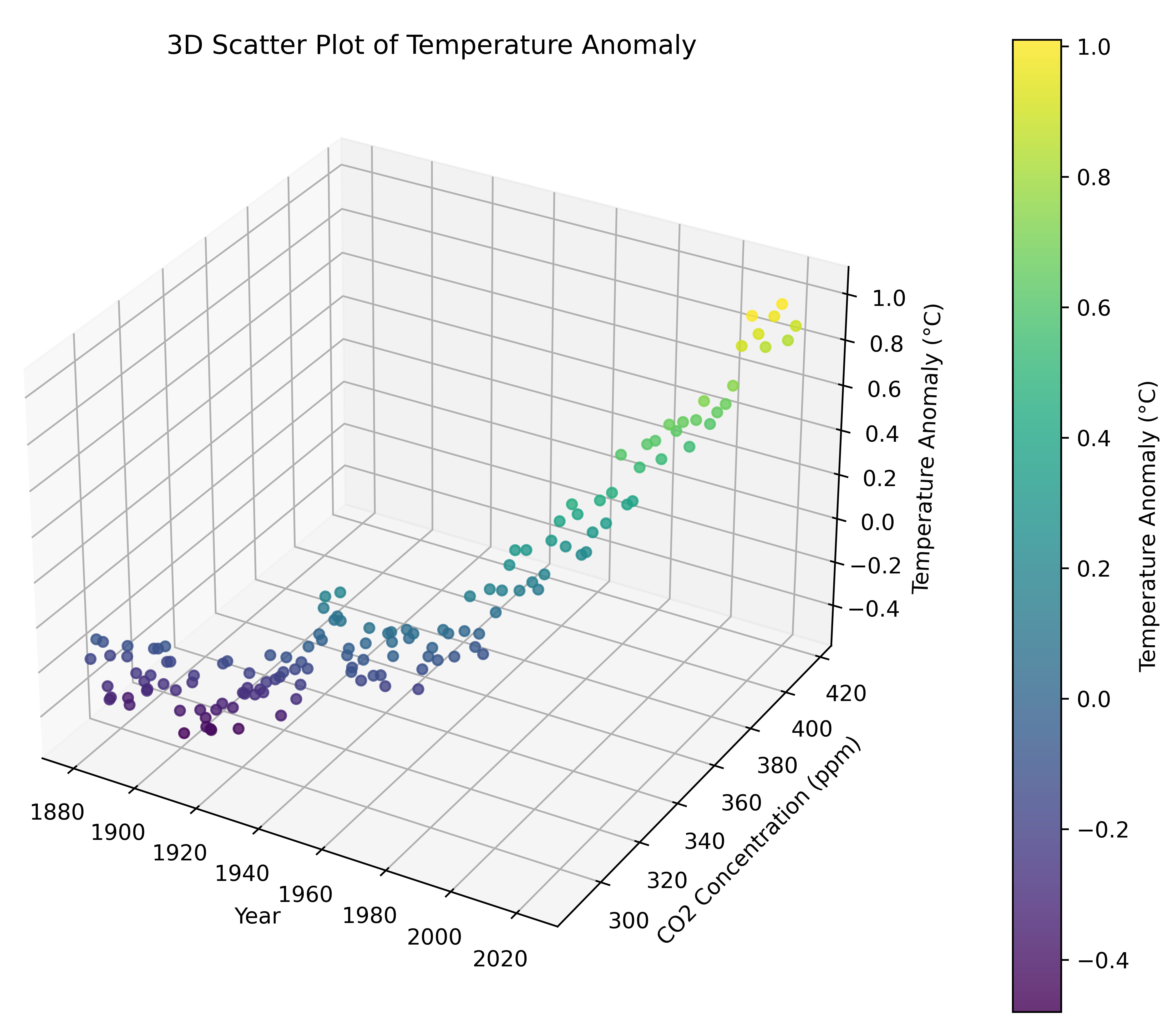
It is bit hard to see in this static view, but if you could rotate and look at this plot from different angles, you would see that the temperature anomaly goes up both with increasing time (year) and with increase CO₂ concentration. Thus, we know in our model that the parameters (weights) of the model, r₁ and r₂, will be positive for both.
Using our new knowledge of vectors and matrices, we can package the parameters of the model into a vector, W = [w₁, w₂]. We can also package the inputs to our model into a vector, X = [time (t), CO₂ (c)].
Then our model is easier to specify as the dot product between W and X. Let’s give the model the short name A(X), since it takes an X and returns the anomaly. Actually, we should call it A(X,W), since it really takes our input vector X and also a fixed parameter vector W, and returns the temperature anomaly. But because W is fixed after training (to be discussed), it generally notated differently. You will see the following notations out in the wild:
A(X), this notation is often used when the parameters are fixed after training, so the parameters are an implicit (hidden) input to the functionA(X,W), this notation highlights the fact that the function A really is a function of both X and W, but its downside is that it does not distinguish between a true variable X and parameters W that are semi-fixed.A(X;W), this notation shows the function A is a function of bothXandWbut separates them with a semi-colon, and everything after the semi-colon is understood to be a parameter.

I have to insert an image to show this last one, but it denotes the parameter vector as a subscript of A, i.e. A_W(X), suggesting that the function A depends on the parameter vector W in a way different than the input X.
I have decided to use the A(X;W) notation in this post, because for didactic reasons it is always best to make as much explicit as possible. So here is our model:
A(X;W) = W ⋅ X + b
Remember, b is the bias (offset, intercept) of the model that serves as a fixed reference point. The dot product when applied yield the same result.
A(X;W) = w₁⋅t + w₂⋅c + b
We can even include b in the vector representation of this model to make it even more compact.
W = [w₁, w₂, b]
X = [time (t), CO₂ (c), 1]
A(X;W) = W ⋅ X
So now we can depict our 2-variable model with a very simple string diagram:
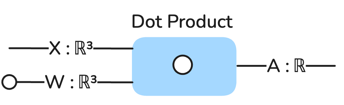
X and W are both vectors of type ℝ³, which just means they are 3-dimensional (length) vectors of real numbers, and remember, real numbers are basically just any arbitrary decimal numbers in machine learning. They are 3-dimensional because we tacked on the bias element needed in each.
This shows that linear algebra concepts can dramatically simplify how to think about and represent models that would otherwise be unwieldy if we had to stick with middle school mathematics.
Training the model
We now know enough mathematics to be able to clearly define a mathematical linear model of mean global temperature anomalies, but in order for the model to make accurate predictions, we need to choose the set of parameters W = [w₁, w₂, b] that best model the data. Now, in 2 or even 3 dimensions, we could choose some representative points and solve a mathematical equation to find w₁, w₂, and b, but as we consider bigger models with more parameters, this approach becomes infeasible. We need an automated procedure to find the optimal set of parameters for any model with any number of parameters and complexity. Such a procedure is called optimization, training, or learning in the machine learning context.
There are many such training algorithms (just another term for an automated procedure), but we will only consider one here as it is the main one used in practice today. It is called gradient descent (also historically called backpropagation in the neural network context specifically).
First, we need to take a step back. If we plot the data, pick some representative points, draw a line between them, and then figure out the parameters, we are implicitly deciding how accurate the model is by deciding which points are most representative. If we picked a random set of points to draw a line between, we have an intuitive sense of how well those points represent the broader data, i.e., how well the model fits the data.
Implicitly, we have an objective function (also called and error, loss or cost function).
An objective function is a function that takes a model and returns a number indicating how accurate (or equivalently how inaccurate) the model is, i.e. how well it represents the data. Hence, it is a function whose input is a function. It essentially rates the quality of a machine learning model. For any given model, you could define any number of different kinds of objective functions. But simple is better.
One of the simplest objective functions we could define is called the Mean Absolute Error (MAE), which is defined as:

What does that equation say? Well, our climate linear model A(X;W) takes a vector X and returns it’s predicted temperature anomaly. In the machine learning field, the ground truth is usually called y, and the model prediction for y is called “y hat” or ŷ. So ŷ is the same as A(X;W) for some given input vector X.
If you have a set of pairs of (ŷ, y) data points generated from your model, then you take the absolute difference |ŷ - y| between each pair, add them all up, and then divide by the number of data pairs, and that is the mean absolute error (MAE).
For example, let’s say X = [x₁, x₂] = [2018, 407], that is, we want the model to tell us what the temperature anomaly was for the year 2018, assuming the CO₂ was 407 ppm. But in order for the model to give us an accurate answer, it needs to know the appropriate weights (parameters) W, so training (optimizing) the model is the process of finding the optimal parameter vector W that will give us accurate answers for some input vectors X.
We start with a blank slate parameter vector W by initializing it to random numbers, so the model is going to make a prediction, and that prediction is A(X;W) = ŷ, and the ground truth (what the actual temperature anomaly was for 2018) is y. In this case, y = 0.85.
Since we already know that the temperature anomaly has been increasing over time since 1880 and we know that higher CO₂ concentrations causally contribute to a higher temperature anomaly, we know the parameters w₁ and w₂ are going to be positive numbers, so we can initialize W to be a set of random but positive numbers.
Data Preparation
There’s an issue we need to solve before we can continue with introducing the training procedure, however.
Let’s just pick some small random positive numbers between 0 and 1, e.g. w₁ = 0.1, and w₂ = 0.6. We will initialize b = 1. So W = [0.1, 0.6, 1].
Let’s see what happens if we plug these into our model.
X = [2018, 407, 1], W = [0.1, 0.6, 1]
A(X;W) = 0.1 * 2018 + 0.6 * 407 + 1 = 447.
The answer we get from our model is supposed to be a temperature anomaly in degrees celcius, and we just got 447. That number is so outrageously large, it’s not even in the right order of magnitude. The true answer is y = 0.85.
What can we do to at least get our model in the right order of magnitude? Well, we could make b really big. If we initialize b = -440, for example, then we get:
X = [2018, 407, 1], W = [0.1, 0.6, -440]
A(X;W) = 0.1 * 2018 + 0.6 * 407 - 450 = 6.
At least we’re close to the right order of magnitude, but now our parameter vector contains parameters that are of different order of magnitudes, and this turns out to make training the model more challenging than it needs to be. When the parameters have very different sizes, it becomes very sensitive to small changes in some of the parameters, making training unstable.
Hence, we need our parameters to be in a similar size range. So rather than try to fiddle with the parameters, we’re going to modify our dataset. We cannot change the meaning of our data, we have to keep it in the same mathematical space (as described earlier), but we can change the number ranges without changing the meaning by standardizing the data. This will make the data all in a similar range. Standardizing is done by running the data through this function:

The input to this function is a vector X, e.g. X = [92, 2, 190, -5, 0.8, 9025] (i.e. numbers with a wide range of sizes), and computes this transformation:
X = [92, 2, 190, -5, 0.8, 9025]
Mean(X) = 1550.8
Standard Deviation of X = std(X) ≈ 3343
Centered X = [92, 2, 190, -5, 0.8, 9025] - 1550.8 = [-1458.8, -1548.8, -1360.8, -1555.8, -1550. , 7474.2]
Centered X / std(X) = [-1458.8, -1548.8, -1360.8, -1555.8, -1550. , 7474.2] / 3343 =
S(X) = [-0.44, -0.46, -0.41, -0.47, -0.46, 2.24]
We started with a vector (list) of numbers ranging from -5 to 9025, and now after standardization, the range is from 0.47 to 2.24, so all within a much more reasonable range. We will need to do this with our temperature anomaly data, and this is what we get:
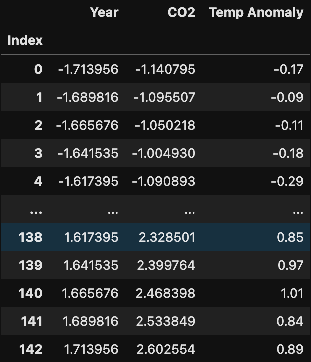
We’ve transformed the time variable (which was in years) into a scale that can range from a small negative number to a small positive number, and the same with the CO₂. This makes training much easier.
I should point out there is a related concept to standardization called normalization, and normalization refers to transforming some data to be within a specific range, for example, forcing some data to be in the range 0 to 1.
In any case, this kind of data preparation or data pre-processing is often necessary for machine learning models.
Back to Training
Now that our data is prepared properly, we can get back to figuring out how to train (optimize) the A(X;W) model.
Let’s get back to starting with X = [2018, 407, 1], or after standardization…

X = [1.62, 2.33, 1] (rounded)
Let’s keep W = [0.1, 0.6, 1] and see what happens now.
A(X ;W) = 0.1 * 1.62 + 0.6 * 2.33 + 1 = 2.56
Hooray, 2.56 is at least in the ballpark.
Let’s use our Mean Absolute Error (MAE) objective function to get the loss (error, cost) of the model for this input.
MAE(X) = |ŷ - y| = 2.56 - 0.85 = 1.71
(Since we only have one data point, we’re not actually computing a mean absolute error but just an absolute error, but let’s just still call it the MAE to be consistent.)
Our model is over-estimating y (ground truth) by 1.71, so we want to nudge the model parameters such that the prediction will be lower for this X. How can we do this?
Well, we have 3 choices, we can lower w₁, w₂, or b. How do we know which one? At this point, there’s no way to know, so let’s just pick w₂ to lower. Let’s lower it from 0.6 to -0.13 and recompute A(X;W).
A(X ;W) = 0.1 * 1.62 + (-0.13 * 2.33) + 1 = 0.8591
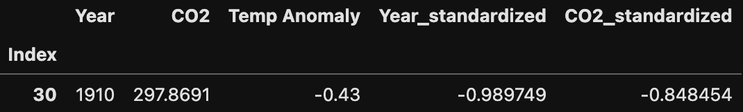
Okay, so that’s very close to the ground truth, in this case |ŷ - y| = 0.0091, which is pretty small. So are we done, is our model trained? No, definitely not, we just optimized the model with respect to a single data point from our training dataset. Our new parameter vector is w = [0.1, -0.13, 1], so let’s see how our model performs with a different input x = [1910, 298] = [-0.99, -0.848] (after standardization). The ground truth temperature anomaly is y = -0.43.
A(X ;W) = 0.1 * (-0.99) + (-0.13 * -0.848) + 1 = 1.01
Now our absolute difference is ŷ - y = 1.01 - (-0.43) = 1.44
Our model is back to over-estimating again, but with a different input.
But we can’t just decrease any of the parameters because that will affect the previous data point we gave it for year 2018.
We need a way to optimize W that will lower the MAE for both X, year = 2018 and X, year = 1910.
So here’s what we’ll do, we will compute the MAE for both of these data points together, and we will systematically nudge each parameter up and down a little bit to see if it either increases or decreases the MAE.
Let’s label X₁ to be the data for year 1910 = [-0.99, -0.848, 1]
And X₂ is the data for year 2018 = [1.62, 2.33, 1]
The starting (baseline) MAE for these two points is:
MAE(X₁,X₂) = (1/2) * ((ŷ₁ - y₁) + (ŷ₂ + y₂))
Where ŷ₁ is the model prediction for X₁ and ŷ₂ is the model prediction for X₂.
If we start with our initial random W = [0.1, 0.6, 1], then
(ŷ₁ = 2.56, y₁ = 0.85) and (ŷ₂ = 0.3922, y₂ = -0.43)
MAE(X₁,X₂;W) = 0.5 * ((2.56 - 0.85) + (0.3922 - (-0.43))) ≈ 1.27
So the total error (MAE) for both of these two data points, given a randomly initialized W, is about 1.27. Now the question is, how can we update (optimize) the components of the W vector to minimize the MAE? We want the MAE to be as close to 0 as possible.
We’re going to create an iterative trial-and-error training algorithm that we will call the iterative nudge training algorithm.
Let’s choose a small number, we’ll call it delta and use the greek delta symbol δ, and set δ = 0.1.
Next, let’s iterate through each of the parameter components of W and nudge each one up by either a positive or negative δ (0.1). Then after doing these two nudges in opposite directions, we will recompute the MAE for the two new W’s that we’ll call W₊ (W plus) and W₋ (W minus) and we will see if W₊ or W₋ made the MAE lower. We will do that for each of the 3 parameters, and that should tell us whether to nudge up or down each parameter. If we repeat this process many times with a small enough δ, then eventually our MAE should get close to 0, because W will be optimized (trained). At least for these 2 data points.
Let’s begin.
W = [0.1, 0.6, 1], recall, baseline MAE = 1.27
W₊ = [0.1 + 0.1, 0.6, 1] = [0.2, 0.6, 1]
MAE(X₁,X₂;W₊) = 1.2976 (Calculations not shown.)
W₋ = [0.1 - 0.1, 0.6, 1] = [0, 0.6, 1]
MAE(X₁,X₂;W₋) = 1.2346
Therefore, we should keep W₋ since its associated MAE is a bit lower.
Now we do the same for the second component, while retaining the others.
W₊ = [0.1, 0.6 + 0.1, 1] = [0.1, 0.7, 1]
MAE(X₁,X₂;W₊) = 1.34 (Calculations not shown.)
W₋ = [0.1, 0.6 - 0.1, 1] = [0.1, 0.5, 1]
MAE(X₁,X₂;W₋) = 1.19
Therefore, we keep W₋ again since its associated MAE is a bit lower.
Now we do the same for the third component, while retaining the others.
W₊ = [0.1, 0.6, 1 + 0.1] = [0.1, 0.6, 1.1]
MAE(X₁,X₂;W₊) = 1.37 (Calculations not shown.)
W₋ = [0.1, 0.6, 1 - 0.1] = [0.1, 0.6, 0.9]
MAE(X₁,X₂;W₋) = 1.17
Therefore, we keep W₋ again since its associated MAE is a bit lower.
Now we’re done with this first iteration, the final new W we get is
W' = [0.1 - 0.1, 0.6 - 0.1, 1 - 0.1] = [0, 0.5, 0.9]
MAE(X₁,X₂;W’) = 1.06
So through this iterative trial-and-error process, we decreased the MAE from 1.27 to 1.06.
If we ran through this procedure a few more times, we could get the MAE lower and lower. In fact, I have an algorithm in Python to do just that:
import numpy as np

def compute_mae(X, y, W):
    """
    Compute the Mean Absolute Error (MAE) for a linear model.

    Parameters:
    - X: input data (n_samples, n_features)
    - y: true target values (n_samples,)
    - W: model parameters [w1, w2, ..., b] (n_features + 1,)

    Returns:
    - MAE: float
    """
    return np.mean(np.abs(np.dot(X, W[:-1]) + W[-1] - y))

def train_with_nudges(X, y, W, delta=0.1, iterations=10):
    """
    Train model parameters using iterative nudges.

    Parameters:
    - X: input data (n_samples, n_features)
    - y: true target values (n_samples,)
    - W: initial model parameters [w1, w2, ..., b] (n_features + 1,)
    - delta: nudge size
    - iterations: number of passes over parameters

    Returns:
    - W: optimized parameters
    """
    for _ in range(iterations):
        for i in range(len(W)):
            W_up, W_down = W.copy(), W.copy()
            W_up[i] += delta
            W_down[i] -= delta
            if compute_mae(X, y, W_up) < compute_mae(X, y, W):
                W = W_up
            elif compute_mae(X, y, W_down) < compute_mae(X, y, W):
                W = W_down
    return W

# Example
X = np.array([[1.62, 2.33], [-0.99, -0.848]])  # Standardized inputs
y = np.array([0.85, -0.43])                    # Ground truth
default_W = np.array([0.1, 0.6, 1.0])          # Initial parameters

# Initial MAE
print(f"Initial MAE: {compute_mae(X, y, default_W):.4f}")

# Train
optimized_W = train_with_nudges(X, y, default_W, delta=0.1, iterations=10)

# Final MAE
print(f"Final MAE: {compute_mae(X, y, optimized_W):.4f}")
print(f"Optimized Parameters: {np.around(optimized_W, 2)}")
You do not need to understand the code at this point, but I thought I would include it for those who know some Python. Here’s the output we get:
Initial Mean Absolute Error: 1.2661
Final Mean Absolute Error: 0.0438
Optimized Parameters: [0.1 0.3 0. ]
Now this was trained using only 2 data points, let’s see what we get when we run the same training process over all the data with a randomly initialized parameter vector W.
# Training Run 1
Initial MAE: 0.8832
Final MAE: 0.1104
Optimized Parameters: [0.14 0.18 0.05]
Now we can use this trained set of parameters to predict out into the future if we know what the CO₂. For example, our data set ends at year 2022, but we easily look up that the CO₂ concentration in 2023 was 420 ppm (standardized to be 2.70), and the temperature anomaly was about 1.08°C. The standardized year for 2023 is 1.74. Our model predicts:
A(X;W) = 0.14 × 1.74 + 0.18 × 2.70 + 0.05 = 0.78
Let’s try re-running the algorithm again with differently initialized parameter vector W.
# Training Run 2
Initial MAE: 0.9107
Final MAE: 0.0941
Optimized Parameters: [0.01 0.34 0.05]
A(X; W) = 0.01 × 1.74 + 0.34 × 2.70 + 0.05 = 0.99
This is good, 0.99 is pretty close to the ground truth of 1.08, so at first pass our model is at least on the right track. Interestingly, with this second run we get a similar initial and final MAE, but the optimized parameters are significantly different, why?
Well this is a good opportunity to discuss the problem of multicollinearity.
Let’s break down the term, “multi” meaning many or multiple, “co” meaning together, and “linearity” (something we learned earlier). Basically it’s when we have multiple inputs that are linear together, or in other words, multiple inputs that are highly correlated (i.e. they share very similar information).
For example, if you try to build a linear model that predicts someone’s height using their left and right leg lengths as inputs, the model will suffer from multicollinearity because the left and right leg are almost certainly going to be co-linear (carry the same information), since they are probably the same exact length.
Height = c₁ ⋅ right_leg + c₂ ⋅ left_leg + b
We know that right_leg ≈ left_leg, or in other words, right_leg = left_leg + small_error.
Plugging this back into the equation…
Height = c₁ ⋅ (left_leg + small_error) + c₂ ⋅ left_leg + b
Height = c₁ ⋅ left_leg + c₁ ⋅ small_error + c₂ ⋅ left_leg + b
Since c₁ is just some fixed number, and small_error is just some fixed number, we can recombine these with the offset parameter b, which is also just some fixed number.
That is, d = c₁ ⋅ small_error + b
Therefore, Height = c₁ ⋅ left_leg + c₂ ⋅ left_leg + d
Then we can factor out left_leg and get:
Height = (c₁ + c₂) ⋅ left_leg + d
Now we could train this model on some data to find the optimal [c₁, c₂, d] parameters to predict someone’s height from their left leg length, but instead of c₁ and c₂ being unique solutions, c₁ and c₂ can be anything as long as their sum is the same.
In other words, the model could decide to use 10% of the information from the left leg and 90% of the information from the right leg and sum them together, or 50% and 50%, or any such combination.
Multicollinearity transforms what should ideally be a unique solution for the model parameters into a set of equally valid solutions.
In the climate model case, the problem is Year and CO₂ both increase over time, they are very co-linear. So what we should do, is drop out year, and just try to predict the temperature anomaly from the CO₂ concentration, or add in something else that could be helpful (such as total solar irradiance or another greenhouse). In fact, in the second re-training of the model, the training algorithm essentially drops out year by setting the first parameter close to 0.
To clarify some notation, X is a vector representing a single data point [Year, CO₂, 1] (the 1 at the end is added for the bias) and W is a vector representing the parameters of the model [w₁ , w₂ , b]. Therefore, X and W are both vectors of real (decimal) numbers in 3 dimensions, written as:
X : ℝ³ and W : ℝ³
The training points X each have 2 predictors (also called features) Year and CO₂. In more complex models, the number of features or predictors denoted p can be quite large.
Batch Training and a bit more linear algebra
With the current iterative nudge training algorithm we iterative through each individual training point. In our data set we have n = 143 data points.
We can package all the data into a training matrix by stacking them into rows. Since each data point has 2 predictors plus 1 for the bias, we can build a matrix that has n rows and 3 columns. To distinguish vectors from matrices, we will bold a letter if it’s a matrix.
X : ℝⁿᐧᵖ
This notation means that X is a matrix of real (decimal) numbers with dimensions n × p. Since the parameter vector is always going to have the same number of parameters as there are predictors (features) plus the bias, the length of W will always be the same length as each row in X. In other words, if X : ℝⁿᐧᵖ then W : ℝᵖ. Therefore we can compactly represent the model and its computation over all the datapoints simultaneously as:
A(X;W) = X⋅W
That is, we multiply the data matrix with the parameter vector. The output we get will have the dimensions n, that is, we will get a vector of predictions for the temperature anomalies for each of the n training data points. When multiplying matrices and vectors (or tensors more generally), the dimensions must type match. The best way to think about this is in terms of string diagrams.
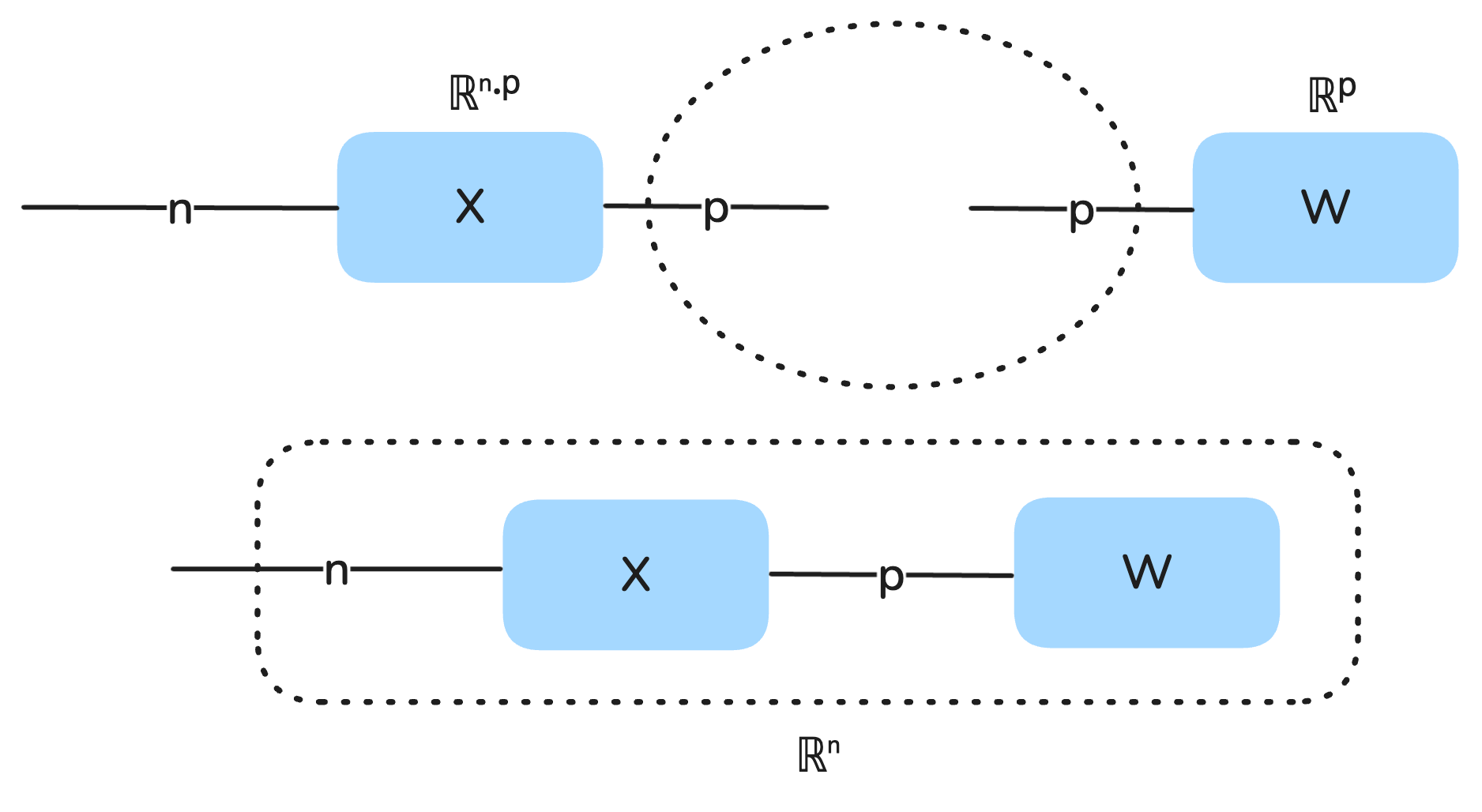
We can visualize a tensor as a string diagram where there is a box and 0 or more “strings” emanating from the box, and each string as a size or dimension. A vector has one dimension so it has one string. A matrix has two dimensions so two strings. Only when one of the matrix dimensions matches the vector dimension can they be multiplied (they type match), and that is visually represented as the compatible strings binding together, leaving just one dangling string that represents the remaining dimension. So a matrix-vector product is always a vector.
Summary
In Part 3, we explored how linear algebra concepts like vectors, matrices, and dot products directly enable machine learning models to represent and manipulate data. Using these tools, we extended our temperature anomaly model to include multiple variables—like CO₂ concentrations—and packaged the inputs and parameters into vectors, simplifying the representation of our model.
We also introduced the process of training a model, where we adjust its parameters to minimize error using an objective function, such as Mean Absolute Error (MAE). Through a hands-on example, we saw how an iterative, trial-and-error approach, akin to gradient descent, allows us to systematically nudge model parameters to improve accuracy. Along the way, we tackled real-world considerations, like standardizing data to ensure stable training.
In part 4, we will formally make the connection between this simple training procedure and gradient descent, which is the true training workhorse of modern deep learning.