


Neural Networks Less Hard - Part 5
An introduction to neural networks anyone can understand.

Recap of part 4
In Part 4, we introduced the concept of differentiation and how it’s used to optimize machine learning models. We started with simple examples, like f(x) = x² and f(x) = x³ − 3x, and showed how derivatives can identify points where a function reaches a minimum or maximum. We then extended these ideas to higher dimensions using partial derivatives, like ∂f/∂x and ∂f/∂y for functions of multiple variables. Finally, we derived the gradient of the mean squared error (MSE), ∇MSE(X, y; W), and explained how it tells us the rate and direction of change in error with respect to the model parameters W. This set the stage for gradient descent, where parameters are updated using the rule W = W − η ⋅ ∇MSE(X, y; W), with η controlling the step size. Gradient descent is faster and more scalable than the iterative nudge algorithm from Part 3, and it forms the backbone of modern machine learning optimization.
Training using Gradient Descent
Let’s recall the problem setup:
We start with a dataset X : ℝⁿˣᵖ, where n is the number of data points, and p is the number of features (or predictors). In this example, X includes two features: the standardized year and CO₂ concentration. We also have y : ℝⁿ, which represents the true target values for the data points (temperature anomalies). Finally, we have a parameter vector W : ℝᵖ, which includes weights w₁, w₂, …, wₚ, as well as a bias term b, treated as part of W.
To ensure the bias term is handled consistently, we modify X by adding a column of ones, turning it into a matrix X : ℝⁿˣ⁽ᵖ⁺¹⁾. This allows the bias b to be incorporated seamlessly into the parameter vector W : ℝ⁽ᵖ⁺¹⁾.
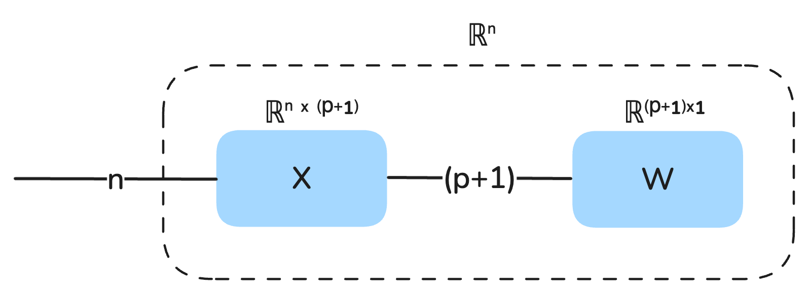
Our model is represented as a string diagram:
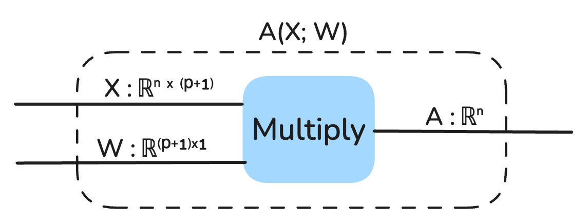
We can also view the output of the model as a static vector that is composed of the multiplication of X and W:
Our goal is to minimize the mean squared error (MSE) of the model. The MSE is a measure of how far off the model’s predictions are from the true target values and is computed as follows:
Compute the model’s predictions: prediction = X · W, where · represents the dot product.
Calculate the residuals, or errors, as residual = y − prediction.
Square each residual, sum them across all n data points, and take the mean.
Once we have the MSE, we calculate its gradient ∇MSE : ℝ⁽ᵖ⁺¹⁾, which gives the rate of change of the MSE with respect to each parameter in W plus the bias term b. The gradient is computed as follows:
For each feature wᵢ, calculate how much the error changes with respect to wᵢ.
Use the formula:


Instead of explicitly looping and summing through each of the n datapoints, we can actually rewrite the gradient using pure matrix-vector multiplications (sometimes called vectorizing):

I have not explained what the notation Xᵀ means yet. So recall, that X is the matrix of our data, in this case it has 143 rows, with 2 predictors (features) plus a bias term, so it has 3 columns, so we refer to its dimensions as Row x Column, or in this case, 143 x 3. The little ᵀ notation refers to a transposition where we switch the dimensions of the matrix, so that if X : ℝ¹⁴³ˣ³, then this is the transpose Xᵀ : ℝ³ˣ¹⁴³.
Whenever we are doing tensor (remember, that’s the more general term that encompasses scalars, vectors, matrices and high-order arrays) multiplications we need to make sure the dimensions match up.
XW:
X is n × (p+1), W is (p+1) × 1.
Multiplying X by W gives n × 1.
y − XW:
y is n × 1, XW is n × 1.
Subtracting gives n × 1.
Xᵀ(y − XW):
Xᵀ is (p+1) × n, (y − XW) is n × 1.
Multiplying gives (p+1) × 1.
∇MSE = −(2/n)Xᵀ(y − XW):
Xᵀ(y − XW) is (p+1) × 1, and −(2/n) is a scalar.
Scaling preserves dimensions, so ∇MSE is (p+1) × 1.
This matches W, which is (p+1) × 1, so the dimensions match up (i.e. type-check).
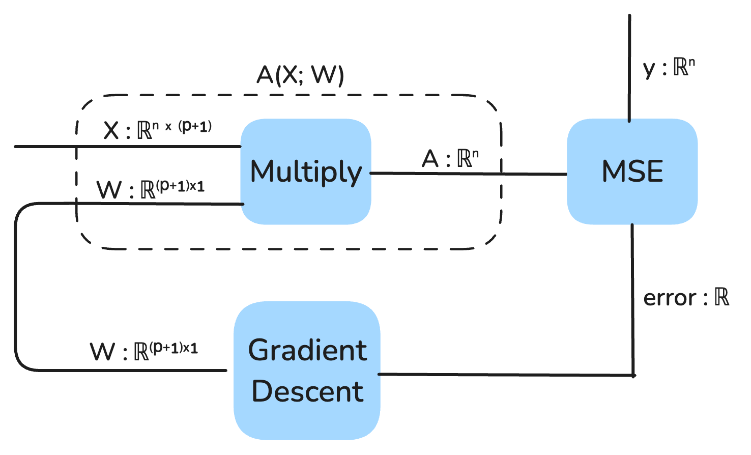
With the gradient in hand, we can perform gradient descent. The key idea is to iteratively update the parameters W in the direction that reduces the MSE. This is done using the update rule:
W = W − η · ∇MSE(X, y; W),
where η (eta) is the learning rate, a small positive number that controls the size of each update step. Common values for η are in the range 0.1 to 0.001, but it depends on the specific problem and how the data are prepared and often needs to be manually played with to find an optimal value. There are also more sophisticated training algorithms beside the simple gradient descent algorithm we are using here where the the learning rate itself is changed over the course of training.
The gradient descent algorithm proceeds as follows:
Initialize the parameters W ∈ ℝ⁽ᵖ⁺¹⁾ with small random values.
Compute the gradient ∇MSE based on the current W.
Update W using the gradient descent rule.
Repeat steps 2–3 for a fixed number of iterations or until the MSE stops improving (called convergence).
By the end of the process, W will have been optimized to minimize the MSE, meaning the model predictions will be as close as possible to the true target values y. The learning rate η ensures that the updates to W are small enough to avoid overshooting the minimum, yet large enough to converge efficiently. If η is too large and the updates overshoot the minimum, it could lead to divergence where the MSE will unexpectedly grow instead of decrease due to unstable training.
At a high level, here is what gradient descent looks like for this model in a string diagram depiction:
Let’s see how this works using the Python programming language:
import numpy as np
import pandas as pd

def compute_mse(X, y, W):
    """
    Compute the Mean Squared Error (MSE) for a linear model.

    Parameters:
    - X: 2D numpy array of shape (n_samples, n_features)
    - y: 1D numpy array of shape (n_samples,)
    - W: 1D numpy array of shape (n_features,), parameter vector.

    Returns:
    - MSE: float
    """
    predictions = np.dot(X, W)  # Linear model prediction
    errors = y - predictions  # Residuals
    mse = np.mean(errors**2)  # Mean squared error
    return mse

def compute_mse_gradient(X, y, W):
    """
    Compute the gradient of the Mean Squared Error (MSE) with respect to W.

    Parameters:
    - X: 2D numpy array of shape (n_samples, n_features)
    - y: 1D numpy array of shape (n_samples,)
    - W: 1D numpy array of shape (n_features,), parameter vector.

    Returns:
    - gradient: 1D numpy array of shape (n_features,)
    """
    n = len(y)  # Number of data points
    predictions = np.dot(X, W)  # Linear model prediction
    errors = y - predictions  # Residuals
    gradient = -2 / n * np.dot(X.T, errors)  # Gradient of MSE
    return gradient

def train_with_gradient_descent(X, y, W, learning_rate=0.01, iterations=1000):
    """
    Train model parameters using gradient descent.

    Parameters:
    - X: 2D numpy array of shape (n_samples, n_features)
    - y: 1D numpy array of shape (n_samples,)
    - W: 1D numpy array of shape (n_features,), initial parameter vector.
    - learning_rate: float, step size for gradient descent.
    - iterations: int, number of passes over the dataset.

    Returns:
    - W: 1D numpy array, optimized parameter vector.
    """
    for _ in range(iterations):
        gradient = compute_mse_gradient(X, y, W)  # Compute gradient
        W -= learning_rate * gradient  # Update parameters
    return W


# Prepare the inputs and target
X = cd2[['Stan_Year','Stan_CO2']].values
y = cd2['Temp Anomaly'].values

# Add a bias term (intercept) to the input data
X = np.hstack([X, np.ones((X.shape[0], 1))])  # Add a column of ones for bias

# Initialize model parameters to match the number of features + bias
W = np.random.rand(X.shape[1])  # Initialize W with the correct shape (p + 1)

# Compute initial MSE
initial_mse = compute_mse(X, y, W)
print(f"Initial MSE: {initial_mse:.4f}")

# Train the model using gradient descent
optimized_W = train_with_gradient_descent(X, y, W, learning_rate=0.1, iterations=100)

# Compute final MSE
final_mse = compute_mse(X, y, optimized_W)
print(f"Final MSE: {final_mse:.4f}")
print(f"Optimized Parameters: {np.around(optimized_W, 2)}")
This code returns the output:
Initial MSE: 2.3050
Final MSE: 0.0132
Optimized Parameters: [0.02 0.33 0.06]
Repeatedly running this code will yield slightly different results each time because the initial W vector is initialized randomly.
With an initially random weight vector W we get a mean squared error of about 2.3, and after 100 iterative updates to W the MSE converges to about 0.01.
If you do not understand the code due to a limited programming background, I recommend you copy-and-paste the code into your favorite state-of-the-art AI chatbot (e.g. ChatGPT, Claude, DeepSeek, etc.) and ask it to explain it to you at your background level.
Let’s look more carefully at the optimized parameters of W. In order, we have w₁ = 0.02 w₂ = 0.33, and b (bias term) = 0.06. Remember our discussion of multi-collinearity from part 3? Well the algorithm learned that Year and CO₂ are co-linear, i.e., they basically share the same information to a large degree, so including both as features (predictors) is redundant.
That is why w₁ is so small, it is almost 0. The bias term is also pretty small, and that is because we already standardized our data so it should be centered around 0 without needing any offset. All this tells us, that to predict the temperature anomaly we really only need to pay attention to the CO₂ concentration. We could have built a much simpler model that is just A(X; w) = w⋅X where X is just a vector of CO₂ concentrations and w is just a single scalar parameter. (I knew this of course before writing this tutorial, and I included the unnecessary complexity for educational purposes.)
The data set I put together for this includes data from 1880 to 2022, so the model was only trained up to 2022. Here is a data point for year 2023: [2023, 420, 1.08], with the features being year, CO₂ concentration in ppm, and the temperature anomaly. Our model expects standardized features, so if we standardize the year and CO₂ we get: [1.744, 2.697, 1.08]. So let’s use our learned W vector and see if it can accurately predict the temperature anomaly for year 2023, i.e. we hope our model produces an output close to the true temperature anomaly of 1.08.
Using the learned parameters 𝐖 = [0.02, 0.33, 0.06] and the standardized 2023 data point 𝐗₂₀₂₃ = [1.744, 2.697, 1], we compute the prediction:
𝐗₂₀₂₃ · 𝐖 = (1.744 × 0.02) + (2.697 × 0.33) + (1 × 0.06)
= 0.0349 + 0.8900 + 0.06
= 0.9849.
The model predicts a standardized temperature anomaly of 0.9849, which is close to the true value of 1.08. This shows the model generalizes reasonably well to unseen data.
Validation and the Problem of Overfitting
What we just did by testing our trained model on a data point (from year 2023) that the model was not trained on, is called validation. We always want to validate the performance of our model on unseen data, usually called test data, to verify it has not just memorized the training data without actually learning a real generalizable pattern. Merely memorizing the training data is called overfitting.
In contrast, underfitting is when the model fails to capture the underlying patterns in the training data, resulting in poor performance on both the training data and unseen test data. Underfitting typically occurs when the model is too simple (e.g., a linear model trying to fit a nonlinear relationship) or when it is not trained sufficiently.
Striking the right balance between overfitting and underfitting is crucial for building a model that generalizes well to new, unseen data. This is why validation, using a separate test dataset, is an essential step in the machine learning workflow.
In the dataset I am using, it has data points for every year from 1880 to 2022, which yields 143 data points. Instead of training the model on all 143 data points, we should only train on say 80% of those (randomly selected), which we will call the training data or set, and the other 20% will be hidden from the model and called the test data or set.
After we have trained the model, we will evaluate how well it did on the held out 20% test data.
Just to make things more confusing, there is also something called the validation set. The validation set is some data that has been withheld from training, that we then assess the trained model on, and depending how it does, we may tweak the model or training algorithm (e.g. the learning rate or other hyperparameters [typically parameters that control the training algorithm itself, not parameters of the model]), and then re-train
The validation set is different from the test set because the test set is what we use once we’ve optimized the model as best we can and we want to know its final accuracy on unseen data. In contrast, the validation set is used to improve model performance indirectly (model tuning). So first we want to see that we can get good model performance on the training data, and then we will assess its performance on the validation data and make tweaks, and finally we will see its performance on the test data. A validation set is not always used, but if it is, then we may split the data into say 70% training data, 10% validation data, and 20% test data.
Since this model is so simple and there is only one hyper-parameter (the learning rate), let’s just do a simple 80%/20% train-test split and see how it performs. Again, this means we take a random 80% subset of the data and use that for training, and leave the remaining 20% just to test the performance of the model without training.
Initial MSE (Training): 1.1844
Final MSE (Training): 0.0134
Test MSE: 0.0126
Optimized Parameters: [0.01 0.34 0.05]
That is the output I get (code not shown). The final training mean squared error was about 0.01 and the final test MSE was about 0.01, so that is exactly what we want to see. If the training MSE was low, but the test MSE was significantly higher, then that suggests the model overfit the training data and does not generalize well to unseen data.
Summary
In this post, we explored the core concepts of gradient descent and its application in optimizing machine learning models. We derived the gradient of the mean squared error (MSE) and explained how it guides parameter updates in the direction of error reduction. We implemented gradient descent in Python, demonstrating how to iteratively update model parameters to minimize MSE. Key takeaways include the importance of the learning rate (η) in controlling update steps and the necessity of testing models on unseen data to ensure generalizability.
Up Next
We now have learned enough foundational skills to actually implement a real neural network, so we will do that in the next parts.