On Computational Graphs

How to derive backpropagation from first principles

Backpropagation is the main training method for neural networks but is often taught without clear motivation. Here I explain how to derive backpropagation from the chain rule in calculus.

Assumptions:

I assume you remember some high school calculus on taking derivatives, and I assume you already know the basics about neural networks and have hopefully implemented one before.

Calculus’ chain rule, a refresher

Before I begin, I just want to refresh you on how chain rule in calculus works. You can skip this section if you are very familiar with the chain rule already.

In calculus, we learn rules about finding the derivatives of functions, such as f(x) = x². The derivative of this function is sometimes denoted f'(x) or using the fraction-like Leibniz-notation df/dx. There is a rule that tells us df/dx = 2x for this function.

Chain rule is the process we can use to analytically compute derivatives of composite functions. A composite function is a function of other functions. That is, we might have one function f that is composed of multiple inner or nested functions.

For example,

is a composite function. We have an outer function f, an inner function g, and the final inner function h(x). To compute this function, we first compute what h(x) is, feed that result into the function g(…), compute that result and feed it into f(…) to get the final answer.

Usually in this case we want the derivative df/dx, and to compute this, we need to compute the derivatives of each of the nested functions and multiply them together, i.e.

More concretely, let’s say

we can decompose this function into 3 separate functions:

or what it looks like as a nested function:

And to get the derivative of this function with respect to x, df/dx, we use the chain rule:

So in each of these cases, I just pretend that the inner function is a single variable and take the derivative as such.

Similarly, you can rewrite the composite function f(x) = e^(sin(x²)) by creating some temporary, substitution variables u = x², v = sin(u), then f(v) = eᵛ and you can use chain rule as above. First you compute df/dv, then dv/du, lastly get the derivative of du/dx. What we ultimately want is df/dx, so we can pretend these derivatives are like fractions, and multiply them such that things cancel out appropriately.

Computational graphs

A computational graph is a representation of a composite function as a network of connected nodes, where each node is an operation or function.
They may be similar in appearance to some graphical depictions of feedforward neural network, but they represent different things. When we visualize these graphs, we can easily see all the nested relationships and follow some basic rules to come up with derivatives of any node we want.

Let’s visualize the above simple composite function as a computational graph.

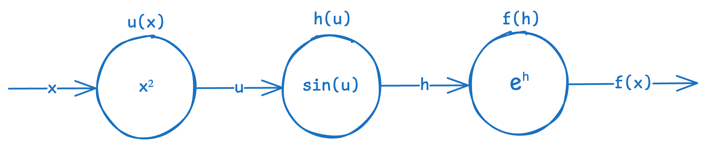
As you can see, from the left to to the right, the graph shows what inputs get sent to each function. Every connection is an input, and every oval shape (called a node) is a function or operation (used here interchangeably). Inside each oval shape (node) is the particular function or operation. The notation above each node is just the function or operation name I’ve arbitrarily assigned.

What’s neat about these graphs is that we can visualize chain rule. All we need to do is get the derivative of each node with respect to each of its inputs.

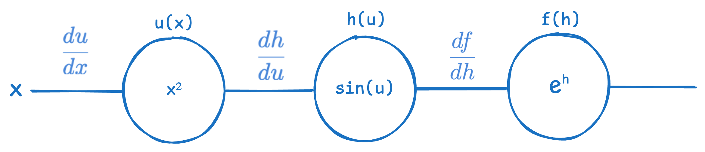
Now you can follow along the graph and do some dimensional analysis to compute whichever derivatives you want by multiplying the ‘connection’ derivatives (derivatives between a pair of connected nodes) along a path. For example, if we want to get df/dx, we simply multiply the connection derivatives starting from f all the way to back to x, which gives us the same equation as the chain rule formula above:

Re-imagining neural networks as computational graphs

An artificial neural network, in the sense of terms like machine learning, deep learning or artificial intelligence, is loosely inspired from real biological neural networks, but in my opinion trying to understand them by analogy to biology is counterproductive. The situation is much simpler actually. An artificial neural network is essentially a massive nested composite function. Each layer of a feedforward neural network can be represented as a single function whose inputs are a weight vector and the outputs of the previous layer. A simple feedforward neural network is really no more complex than the composite f(x) function we just looked at.

This means we can visualize a neural network as a computational graph, and this will allow us to derive the backpropagation algorithm.

Here’s the conventional visualization of a 3 layer neural network (1 input layer, 1 hidden layer, 1 output layer), which could be used to learn very simple problems:

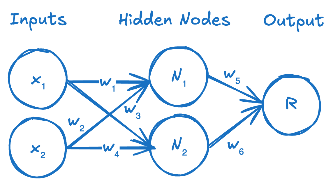
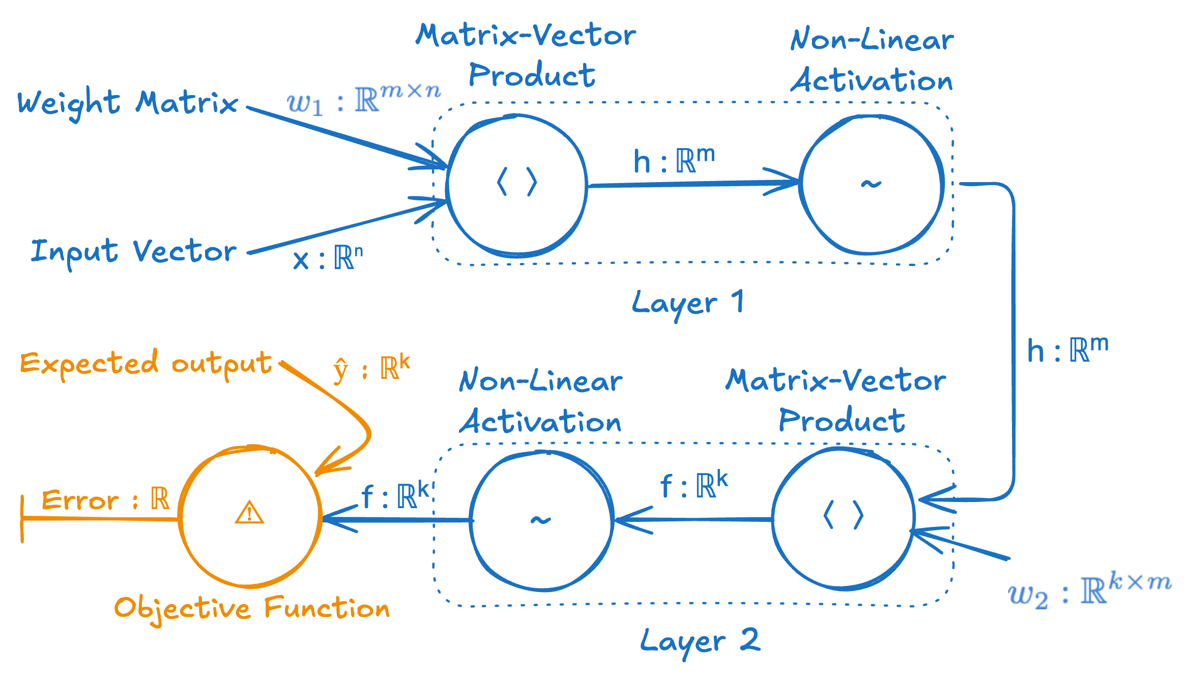
It’s a very intuitive and convenient representation of a neural network in terms of the information flow through the network. However, I don’t think it’s the best way to think about it or visualize it in terms of a computational implementation. We’re going to try re-visualizing this as a computational graph, such that each node is no longer an abstract “neuron” with weights modulating the connection to other neurons, but instead where each node is a single computation or operation and the arrows are no longer weighted connections but merely indications of where inputs are being sent.

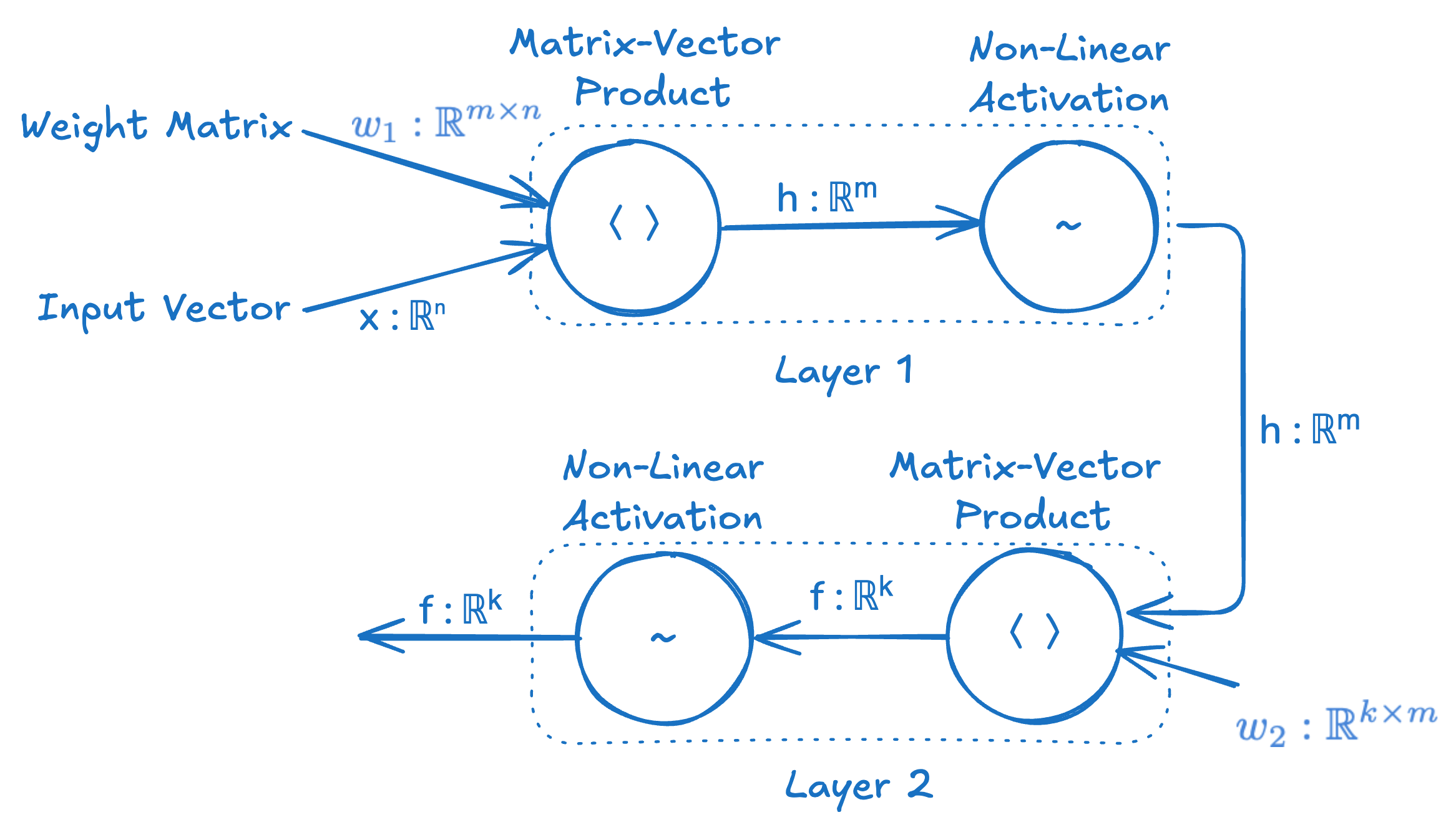
This may look more complex than the traditional neuron-focused depiction of a neural network, but it’s really not, and it tells you exactly how to implement this neural network in code. It shows the step by step functions that occur and the inputs those functions operate on. It also shows the types of all the data flowing through this computational graph.

Here’s how we can implement this simple neural network in Julia, directly translating from this diagram.

# Define activation function
function relu(x)
    return max.(0, x) # Element-wise ReLU
end

# Define the two-layer neural network
function two_layer_nn(x, w1, w2)
    # Layer 1: Matrix-vector product and non-linear activation
    h = relu(w1 * x)
    
    # Layer 2: Matrix-vector product and non-linear activation
    f = relu(w2 * h)
    
    return f
end

# Example usage
# Dimensions: Input vector x ∈ ℝⁿ, 
# weights w₁ ∈ ℝᵐˣⁿ, w₂ ∈ ℝᵏˣᵐ
n, m, k = 100, 10, 2  # Example dimensions
x = randn(n)       # Input vector
w1 = randn(m, n)   # Weight matrix for Layer 1
w2 = randn(k, m)   # Weight matrix for Layer 2

# Compute the output
output = two_layer_nn(x, w1, w2)
println("Output of the two-layer neural network: ", output)

If we want to train this neural network, we need to do so by gradient descent, which involves taking the partial derivatives of the neural network with respect to its parameters (the “weights”).

Actually, we first need an objective function (aka cost function or error function) that tells us how well the neural network is performing.

The output of the neural network gets fed into the objective function, which also needs the expected output ŷ, and it computes a measure of the difference between the actual and the expected output usually called the error or cost.

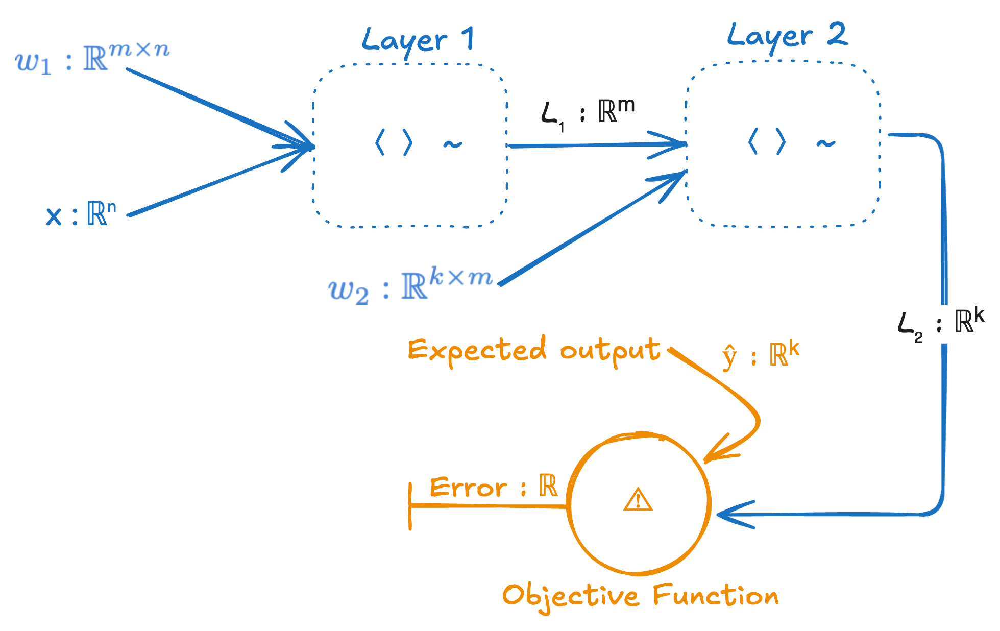
Let’s tidy this up a bit by hiding the details of each layer, and let’s rename h to be L₁ and f to be L₂.

Now let’s show the partial derivatives on this computational graph.

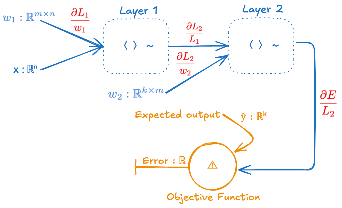
To train this neural network with gradient descent we need ∂E/∂w₁ and ∂E/∂w₂. We can easily find these using the chain rule from calculus.

and

Then the simplest gradient descent learning rule is:

and

Where η is the learning rate.

That is essentially backpropagation. It is just gradient descent by using the chain rule on the composite function that is a neural network. And this is how almost all modern neural networks (deep learning) algorithms are trained.

References

http://colah.github.io/posts/2015-08-Backprop/

https://en.wikipedia.org/wiki/Chain_rule

https://en.wikipedia.org/wiki/Automatic_differentiation

http://www.wolframalpha.com