Sequence Models (NNLH #6)

An introduction to neural networks anyone can understand.

Recap of part 5

In part 5, we explored gradient descent, the core optimization algorithm behind training machine learning models. We built on the concept of differentiation from Part 4, deriving the gradient of the mean squared error (MSE) and used that as the objective function for our temperature anomaly model. We also covered train-test splits and the importance of validation to prevent overfitting, ensuring the model generalizes well to unseen data.

Sequence Models and Probability Theory

We now know enough to build a real neural network, specifically a sequence model. Sequence models are used to handle sequential data, that is, data where there is an inherent time-like ordering, such as language where there is a natural ordering of the letters and words or stock market prices over time. Famous AI applications like ChatGPT are called large language models, and that is just a sophisticated type of a sequence model. What we will learn in this next section will be foundational for understanding LLM’s like ChatGPT.

Let’s consider a language with just 4 letters and 4 words:

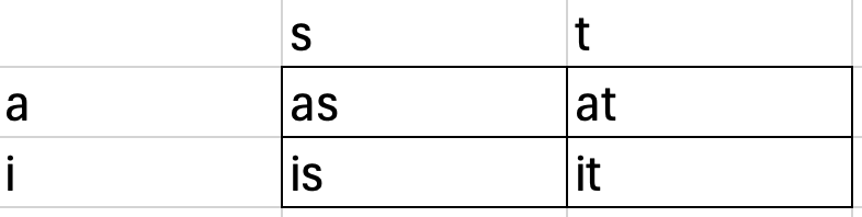
The first column of letters ‘a’ and ‘i’ are the possible first letters, and then each first letter can be paired with a 2nd letter in the set ‘s’ or ‘t’ to form the words: as, at, is, it.

Let’s play a game using these 4 letters and words: if I tell you I’m thinking of a word that starts with the letter ‘a’ and you have to guess which word I’m thinking of, what would you guess?

Well, there are 2 words out of the 4 that start with the letter ‘a’, so you’d h ave to guess it’s either “as” or “at” and since no other information was given, you would have to say there is a 50% chance I’m thinking of “as” and a 50% chance I’m thinking of “at.”

Put more precisely, given I have chosen a word that start’s with the letter ‘a’, the question is: what is the probability of each of the 4 possible words? That is, to make this more mathematically precise, we want to be able to assign a number called a probability that gives us a quantitative way to express how likely each word is, given the starting letter. In this case, since there are only two possible words that start with the letter 'a' ("as" and "at"), and no additional information is provided, we can assign equal probabilities to each of these words. Specifically:

• Probability of “at” = 0.5 (50%)

• Probability of “as” = 0.5 (50%)

• Probability of “is” = 0 (0%)

• Probability of “it” = 0 (0%)

This is because the words "is" and "it" do not start with the letter 'a', so their probabilities are zero in this context.

Probability theory is the mathematical discipline that studies the mathematical structure and use of probabilities, and it is a very complex area. However, for applied machine learning, we can just think of probabilities as representing proportions or frequencies.

The probability of the chosen word being “at” is 0.5 (50%) because there are a total of 2 words that start with the letter “a”, so you just take the quotient 1 / 2 = 0.5. Thus, the probability of some event or outcome is just the number of ways that particular outcome can happen divided by the total number of possible outcomes, given a certain context. Since probabilities are always proportions, they range from 0 (impossible) to 1.0 (certain).

There is a more compact conventional notation for probabilities, where we use a function-like notation P(outcome) = a number in the range 0 to 1. There is also the notation P(outcome | condition) which is read “the probability of ‘outcome’ given some ‘condition’". For example, one could ask what P(tomorrow is sunny | today is sunny). Using this notation:

• P("as" | starts with 'a') = 0.5 (50%)

• P("at" | starts with 'a') = 0.5 (50%)

• P("is" | starts with 'a') = 0 (0%)

• P("it" | starts with 'a') = 0 (0%)

We could also ask P(has an ‘s’), and the answer would be 0.5, since 2 out of the 4 words have the letter ‘s.’

Brief Detour into Set Theory

Before we move on, I need to introduce some more mathematics.

In earlier parts of this series, we introduced notation like y : ℝⁿ, which defines a variable `y` as having the type “real-valued vectors of length n” (i.e. basically lists of decimal numbers).

In mathematics, this would have been written y ∈ ℝⁿ where the symbol ∈ is read as “in.” This is because in conventional mathematics, everything is represented as a set. A set is just some arbitrary collection of things, with no order. This is unlike a list or vector where there is assumed to be a particular order. We usually represent lists and vectors using square brackets, like numbers = [0,1,2,3,4,5,6,7,8,9].

A set is usually denoted using curly braces, for example, here is the set of vowels = {a, e, i, o, u, y}. We can then ask questions like ‘a’ ∈ vowels? And the answer is a boolean True. We can also make statements like g ∉ vowels (the letter ‘g’ is not in the set of vowels).

We can also combine sets using certain set operations, like {a, e, i} ∪ {o, u, y} = {a, e, i, o, u, y}. This is called the union between two sets, which basically combines the sets into one. We can also take the intersection between two sets, such as {a, e, i, o, u, y} ∩ {a, b, c} = {a}, which returns a set containing the shared elements between two sets.

Another operation is the subset operation, e.g., {a, e} ⊂ vowels. There’s also the superset operation, e.g. vowels ⊃ {a, e}. There’s the difference operation (A − B or A∖B) which are the elements in A but not in B.

There’s also the complement operation. Let v = vowels, then vᶜ is the set of non-vowels, assuming that v is part of a bigger set of all letters.

There are others, but the last set operation I want to introduce is the (Cartesian) product: {a, b} × {1, 2} = {(a,1), (a,2), (b,1), (b,2)}, which takes all pairs between each of the two sets.

Technically, most interesting sets in mathematics have an infinite number of elements. For example, the the set of natural numbers (denoted ℕ) which are the numbers {0, 1, 2, 3, 4, …. and so on forever} is an infinite set. In applied machine learning we are generally using the set of real numbers ℝ, which for computers is analogous to the floating point number types. The set of vowels is a finite set.

Everything in a computer is finite. There are no infinite sets on computers because all computers have a finite amount of memory. We can mathematically reason about infinite sets, but once we move to calculating things on a computer, everything is finite.

Back to Probability Theory

When we say P("as" | "starts with a"), we mean that there is a probability function P that assigns a value between 0 and 1 to the specific outcome "as," given that the word starts with 'a'. This is a conditional probability, representing the probability of "as" under the condition that the word starts with 'a'.

To work with probabilities, we must first assume a probability distribution over the parent set of words. We might call this the context or reference set.

A probability distribution is an assignment of a probability to each element of a reference set such that all the probabilities sum to 1.

We could assign probabilities to each element in a reference set in any way we want as long as they all sum to 1. But, there are some standard ways to assign these probabilities that have names such as the uniform distribution, the normal (aka Gaussian) distribution and the Beta distribution.

Let’s assume a uniform distribution, where each word in the parent set is equally likely. Given our example set {as, at, is, it}, the probability of any single word is:
P(word) = 1 / (total number of words) = 1/4 = 0.25.

If we ask for P("starts with a"), this represents the probability that a randomly chosen word starts with 'a'. In this case, "starts with a" refers to the subset of words {as, at}. To compute this we can use the sum rule of probability, which says that for disjoint outcomes (no shared outcomes), P(A ∪ B) = P(A) + P(B), so in our case,
P("starts with a") = P({as} ∪ {at}) = P({as, at}) = P("as") + P("at") = 0.25 + 0.25 = 0.5.

Now, to be clear, whenever we use notation like P({as, at}), we should be writing something like Pᵣ({as, at}), assuming r (reference set) = {as, at, it, is}. We often omit the little subscript that refers to our reference set out of convenience, but the probability function P that maps each element in the set to a probability must do so with respect to some reference set (called the sample space in probability theory) with some assumed probability distribution.

In order to know that Pᵣ(“as”) = 0.25, we have to assume the reference set r has a distribution assigned such that Pᵣ(“as”) = 0.25. It could be possible that we have a different reference set x = {as, ate}, with a different distribution [as ↦ 0.9, ate ↦ 0.1], so when we ask P(“as”) we have to be clear which reference set and distribution we are referring to.

The function P that assigns each element a probability is called a probability mass function (PMF). So Pᵣ is actually a lookup table like this:

+------+-------------+
| Word | Probability |
+------+-------------+
| as   | 0.25        |
| at   | 0.25        |
| is   | 0.25        |
| it   | 0.25        |
+------+-------------+

And when we ask a question like Pᵣ(“as”) we are essentially doing a table (or database) lookup (or query) where we just find the row corresponding to “as” and read off its corresponding probability.

When we ask a question like Pᵣ({as, at}), we find the rows corresponding to “as” and “at” and then sum their corresponding probabilities.

When we ask a question like 𝑃ᵣ("as" | "starts with a"), we first find the rows in the table corresponding to words that start with "a" (the condition). In this case, the relevant rows are:

+------+-------------+
| Word | Probability |
+------+-------------+
| as   | 0.25        |
| at   | 0.25        |
+------+-------------+

From this subset of the table, we normalize the probabilities to ensure they sum to 1, as the condition "starts with a" restricts the reference set to just {as, at}. Normalizing involves dividing each probability by the total probability of the subset, which is:

𝑃ᵣ("starts with a") = 0.25 + 0.25 = 0.5.

Next, we calculate the conditional probability of "as" given "starts with a" by dividing 𝑃ᵣ("as") by 𝑃ᵣ("starts with a"). Using the probabilities from the table:

𝑃ᵣ("as" | "starts with a") = 𝑃ᵣ("as") / 𝑃ᵣ("starts with a") = 0.25 / 0.5 = 0.5.

So, using the table, we determine that under the condition "starts with a," the probability of "as" is 0.5. This process effectively filters the reference set, sums the probabilities for the condition, and normalizes them for conditional probabilities.

Probabilities with Infinite Sets

We learned that a probability mass function like 𝑃ᵣ can return a specific probability value (like 0.02) for whatever question you ask it with respect to the sample space (reference set).

But what about when the sample space is continuous?

For example, let’s say you run an online business on your own server and you want to estimate the probability of a catastrophic server failure. You have implemented strategies to mitigate the risk of that, but you can’t drive the probability of a server failure to 0.

Let’s say you’ve estimated that there is about 1 server failure per year based on historical data, but that server failures are more likely in certain months due to storms that can cause power disruptions. Here’s an example table:

| Month  | Failure Probability |
|--------|---------------------|
| Jan    | 0.05               |
| Feb    | 0.04               |
| Mar    | 0.06               |
| Apr    | 0.07               |
| May    | 0.09               |
| Jun    | 0.12               |
| Jul    | 0.15               |
| Aug    | 0.14               |
| Sep    | 0.10               |
| Oct    | 0.07               |
| Nov    | 0.06               |
| Dec    | 0.05               |

This table suggests that failures are more likely in the summer months (June, July, August) and less likely in winter (e.g. due to summer storms). If failures were evenly distributed, each month would have a probability of 1∕12 ≈ 0.083, but here, July has the highest probability (0.15), while February has the lowest (0.04).

This works fine if we only want to track failures at the granularity of months. But what if we want to ask:

“What’s the probability of a failure occurring on a specific day?”

Now, the monthly probabilities become problematic. If we divide each month’s probability by the number of days in that month, the probabilities get smaller. For example, in July:

𝑃(failure on a specific day in July) = 0.15 ÷ 31 ≈ 0.00484

This is already a small number. If we go further and ask:

“What’s the probability of a failure occurring in a specific hour?”

𝑃(failure in a specific hour in July) = 0.15 ÷ (31 × 24) ≈ 2.01 × 10⁻⁴

And for a specific second:

𝑃(failure in a specific second in July) = 0.15 ÷ (31 × 24 × 60 × 60) ≈ 5.6 × 10⁻⁸

These probabilities become vanishingly small as we decrease the time scale, which is a problem. On a computer, they might underflow and round to zero.

What if instead of tracking the probability of a failure at an exact second, we define failure probability per unit time—in other words, a failure (probability) rate, also known as a probability density.

Density = 𝑃(failure in an interval) ÷ interval length

For monthly failure rates (since each month is approximately 1 ∕ 12 of a year), we compute:

Density in July = 0.15 ÷ (1∕12) = 1.8 failures per year

For a daily failure rate in July:

Density = 0.00484 ÷ (1∕365) = 1.8 failures per year

For an hourly failure rate:

Density = (2.01 × 10⁻⁴) ÷ (1∕(365 × 24)) = 1.8 failures per year

Notice that in every case, the density stays at approximately 1.8 failures per year, regardless of how small the time interval gets.

In contrast, if we check the probability density (failure rate) for a daily in February, we get:

Density = (0.04 failures per month / 28 days in February) / (1 year / 365 days) = 0.52 failures per year, meaning meaning if the entire year had the same failure rate as February, we would expect 0.52 failures in a year.

As an analogy, imagine you're tracking a car as it drives across the country. At a low resolution, it’s easy to say, "The car is currently in California." Zooming in, you can narrow it down to, "The car is in Los Angeles." But what happens if we keep increasing the resolution? If we try to pinpoint the exact location of the car—e.g. down to the nearest meter—it becomes impossible because the car is constantly moving. The moment you report its position, it has already changed.

Instead of asking, "Where is the car exactly?" we start asking, "How fast is the car moving?" This is velocity, and the key advantage is that velocity remains stable at any resolution. If the car is traveling at 70 km/hr, then whether you measure speed per hour, per minute, or per second, the value is still around 70 km/h.

How do we figure out the velocity of the car, well we need to know the distance between two reference points, say position a and position b and we need to know how much time the car took to travel from position a to position b.

Velocity = Duration[a, b] / [b - a]

At increasingly higher resolutions, tracking the car’s exact position becomes meaningless. But, if we know the velocity and we take some time interval, we can easily compute how far the car as traveled.

Distance traveled = velocity × time interval

For example, if the car is moving at 70 km/h, then in 10 minutes it has traveled:

70 km/hr × (10 mins / (60 mins/hr)) = 11.67 km

Probability behaves in exactly the same way when the reference set (sample space) is continuous. At a low resolution, we can say, "There is a 10% chance of a server failure this month." At a higher resolution, we refine it to, "There is a 0.5% chance of failure today." But if we keep zooming in and ask, "What is the probability of failure in the next microsecond?" we run into the same problem as before: the probability shrinks toward zero and becomes meaningless.

Instead of asking, "What’s the probability of failure at this exact second?" we ask, "At what rate are failures occurring?" This is probability density—it tells us how much probability mass there is per some unit length. Just like velocity, probability density remains stable at any resolution.

Probability Density of x = Probability(x being in the interval [a,b]) / [length of the interval a to b]

So in a continuous domain, like continuous time, we do not deal with probability mass functions, but instead probability density functions (PDF).

The notation is a bit confusing because most of the time PMFs and PDFs are both denoted with the letter P.

Unlike raw probabilities which must be some value 0 to 1.0 and the sum of all probabilities from a PMF must equal 1, probability densities can be greater than 1. Instead, PDF’s must integrate to 1. Integration is like summation in the continuous setting. In the continuous setting, we cannot meaningfully ask what the probability of a specific point is, instead, we have to ensure that if we choose any set of non-overlapping intervals over the PDF that the total probability across those intervals must sum to 1.

Mathematically, in the case of a PMF:

Let’s choose some really tiny interval length we will mathematically denote Δx. Then for some point (element) x, the sum of Density(x) ⋅ Δx for all possible values of x will sum to 1.

If we make the interval length Δx smaller and smaller, such that it becomes infinitesimal (for our purposes, an infinitesimal is a symbolic number ε, such that ε > 0 but ε² = 0), then we call this integration. It is essentially summation if you have an infinite number of points (the reference set or sample space is infinite) and the interval length Δx is infinitesimal. We use a different symbol for integration

To make it clear that Δx is infinitesimal, the standard notation switches to dx. Sometimes integrals can be solved algebraically, but often times we approximate the infinite integrals using small but finite intervals.

Back to Sequence Models

Sequence models are functions that predict the next element in sequence given some preceding elements. These elements are often called tokens in the machine learning world.

For example, if I say “The chicken crossed the …” a good textual sequence model would predict the next word (aka element, token) to likely be “road.”

In mathematical (probability theory) terms, this amounts to having a conditional probability distribution over the next words:

P(next word | previous words)

There are many possible next words, so P(next word | previous words) assigns a probability to every possible next word given the previous words. In this case P(next word | “The chicken crossed the …”) would assign high probability to the word “road” and low probability to most other words.

Markov Model

The simplest sequence model we can consider before eventually building neural networks is the Markov model. A Markov model is a model that predicts the next token in a sequence only based on the immediate prior token, i.e. P(next word | previous word).

Here’s a Markov model of the weather:

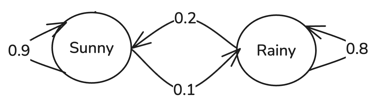
This is a simple Markov model that describes weather transitions between two states: "Sunny" and "Rainy." The model represents these states as circles, with arrows indicating the probabilities of transitioning from one state to another.

Starting from the "Sunny" state, there’s a 90% chance that the weather remains sunny the next day, and a 10% chance it transitions to rainy. Similarly, from the "Rainy" state, there’s an 80% chance that it stays rainy and a 20% chance it shifts to sunny. Each state’s outgoing probabilities add up to 1 (100%), satisfying the basic requirement for a Markov model. The probabilities of transitioning from one state to another are called the transition probabilities.

These transition probabilities can be decided by human expertise or trained (optimized) on some historical (training) data. The transition probabilities can be represented as a matrix called the transition matrix.

Transition Matrix:

        Sunny   Rainy
Sunny   0.9     0.1
Rainy   0.5     0.5

A defining feature of this type of sequence model is that it is memoryless, meaning the probability of transitioning to the next state depends only on the current state, not on how the system got there. For example, if today is sunny, the chance of rain tomorrow is always 10%, regardless of how many sunny or rainy days preceded it.

So let’s say we record whether a day is sunny (S) or rainy (R) in some city over the course of several years up to the present. We then have a dataset composed of a long sequence of S’s and R’s, such as …SSSSSSSSSRRSSSSSSS…

We want to create a computer model that predict what the weather for tomorrow will be, sunny or rainy, based just on the historical data we have.

One way to do that would be to take some fixed context window, and pattern match all instance of that in our historical data, and then simply add up the number of times an S occurs next or an R occurs next and divide by the total, giving probabilities.

For example, let’s say we use a context window of length 2. If today is "SS" (the last two days were sunny), we’d look through the entire dataset and find all instances where "SS" occurred. Suppose we find that after "SS," there were 8 occurrences of "S" and 2 occurrences of "R." Then, based on this pattern, we’d predict tomorrow’s weather as sunny with an 80% probability and rainy with a 20% probability.

If instead the current context is "RS" (yesterday was sunny and the day before was rainy), we’d do the same: search the historical data for all occurrences of "RS" and count what came next. If "RS" is followed by "S" 6 times and by "R" 4 times, the model would predict sunny with a 60% probability and rainy with a 40% probability.

This method essentially builds a probability table based on observed patterns in the data for each possible context. It assumes that the weather tomorrow depends only on the past two days and not on the entire sequence before that. By adjusting the length of the context window, you can balance between capturing more complexity (longer windows) and avoiding overfitting to rare patterns (shorter windows).

The probability table approach works but becomes problematic as the amount of data grow and context window grows. As the context window grows, the number of possible patterns increases exponentially, leading to unreliable or undefined probabilities for rare patterns. It also overfits to noise, predicting with high confidence from limited data, and becomes computationally expensive as patterns grow more complex.

Markov models address these problems by assuming the next state depends only on the current state (or a small fixed history), reducing the state space and generalizing better to unseen sequences. Additionally, once the model is trained then the original training data is no longer needed, thus is dramatically computationally cheaper.

Remember, training (aka optimizing) a machine learning model just means finding the set of model parameters that makes the model perform well.

The parameters of a Markov model are the transition probabilities, which are stored in the transition matrix. The Markov model tells us this:P(xₜ₊₁ | xₜ), which is the probability of next state xₜ₊₁ given the current state xₜ. For the weather example, we want to know P(Sunnyₜ₊₁ | Rainyₜ), which is the probability of it being sunny tomorrow given it was rainy today. We also want to know all 4 other combinations.

A Markov model is both a predictive model and a generative model, depending on how it is used.

A predictive model estimates the probability of certain output data given input data. For example, a trained weather Markov model can tell us how likely it is that tomorrow will be sunny given that today is sunny. Similarly, a machine learning model for digit recognition is predictive because, given an input image, it estimates the probability that a certain region of the image contains a specific number.

A generative model goes further: it can generate new synthetic data that follows the same distribution as the historical training data. A generative Markov model can simulate entirely new sequences of weather patterns, and a generative image model (such as a GAN or VAE) can create novel images that resemble real-world images after being trained on a dataset.

When our 2-state Markov model is used predictively, it computes the conditional probability of the next state given the current state:

P(xₜ₊₁ | xₜ)

For example, if today is Sunny, the model predicts:

P(Sunnyₜ₊₁ | Sunnyₜ) = 0.8, P(Rainyₜ₊₁ | Sunnyₜ) = 0.2

When used generatively, it computes the joint probability of an entire sequence by multiplying conditional probabilities over time:

P(x₁, x₂, …, xₜ) = P(x₁) ⋅ P(x₂ | x₁) ⋅ P(x₃ | x₂) ⋯ P(xₜ | xₜ₊₁)

For example, the probability of generating the sequence Sunny → Sunny → Rainy is:

P(Sunny₁, Sunny₂, Rainy₃) = P(Sunny₁) ⋅ P(Sunny₂ | Sunny₁) ⋅ P(Rainy₃ | Sunny₂)

This comes from the chain rule of probability, which is a fundamental rule that allows us to break down the probability of multiple events occurring together into a sequence of conditional probabilities.

For any sequence of events A₁, A₂, ..., Aₙ, the chain rule states that:

P(A₁, A₂, ..., Aₙ) = P(A₁) ⋅P(A₂ | A₁)⋅ P(A₃ | A₁, A₂)⋅ ... ⋅P(Aₙ | A₁, A₂, ..., Aₙ₋₁).

This formula expresses the joint probability of multiple events as a product of conditional probabilities.

The chain rule comes from the definition of conditional probability, which states that P(A | B) = P(A, B) / P(B).

Rearranging this, we get: P(A, B) = P(A | B) P(B).

Extending this logic to three events, P(A, B, C) = P(A | B, C) P(B, C), and since P(B, C) = P(B | C) P(C), we can expand further: P(A, B, C) = P(A | B, C) P(B | C) P(C). This reasoning extends naturally to any number of events.

In short, predictive Markov models forecast the next state, while generative Markov models generate full sequences by chaining transitions.

This will make more sense later with a specific example.

The easiest way to learn the transition probabilities is to simply count the transitions in the observed data and normalize them.

Count the number of times each transition occurs in the dataset.

• Let C(Sunny → Sunny) be the count of Sunny followed by Sunny.

• Let C(Sunny → Rainy) be the count of Sunny followed by Rainy.

• Let C(Rainy → Sunny) be the count of Rainy followed by Sunny.

• Let C(Rainy → Rainy) be the count of Rainy followed by Rainy.

Compute the transition probabilities by normalizing the counts:

• P(Sunnyₜ₊₁ | Sunnyₜ) = C(Sunny → Sunny) / (C(Sunny → Sunny) + C(Sunny → Rainy))

• P(Rainyₜ₊₁ | Sunnyₜ) = C(Sunny → Rainy) / (C(Sunny → Sunny) + C(Sunny → Rainy))

• P(Sunnyₜ₊₁ | Rainyₜ) = C(Rainy → Sunny) / (C(Rainy → Sunny) + C(Rainy → Rainy))

• P(Rainyₜ₊₁ | Rainyₜ) = C(Rainy → Rainy) / (C(Rainy → Sunny) + C(Rainy → Rainy))

This method maximizes the likelihood of the observed data and gives the maximum likelihood estimate (MLE) of the transition probabilities.

The maximum likelihood estimation (MLE) method finds the transition probabilities that maximize the probability of the observed sequence of states.

Given an observed sequence of weather states:

Sunny → Sunny → Rainy → Sunny → Sunny → Rainy

the likelihood (probability) of this sequence, given the transition probabilities, is:

Likelihood = P(Sunny₁, Sunny₂, Rainy₃, Sunny₄, Sunny₅, Rainy₆) = P(Sunny₁) ⋅ P(Sunny₂ | Sunny₁) ⋅ P(Rainy₃ | Sunny₂) ⋅ P(Sunny₄ | Rainy₃) ⋅ P(Sunny₅ | Sunny₄) ⋅ P(Rainy₆ | Sunny₅)

Since we are estimating transition probabilities, we only maximize the part that depends on them, meaning we can remove the P(Sunny₁) term:

Likelihood = P(Sunny₂ | Sunny₁) ⋅ P(Rainy₃ | Sunny₂) ⋅ P(Sunny₄ | Rainy₃) ⋅ P(Sunny₅ | Sunny₄) ⋅ P(Rainy₆ | Sunny₅)

And since any transition e.g. Sunny → Sunny shares the same probability, the specific time they occur is irrelevant as we just care about the transition probabilities :

Likelihood = P(Sunny → Sunny) ⋅ P(Sunny → Rainy) ⋅ P(Rainy → Sunny) ⋅ P(Sunny → Sunny) ⋅ P(Sunny → Rainy)

The more mathematical looking version of the likelihood is this:

Let’s break this down.

• L is the likelihood, which is the probability of observing the entire sequence given the transition probabilities.

• ∏ (capital pi) represents a product, similar to how ∑ (capital sigma) represents a sum. This means we multiply terms together.

• t=1 to T−1 means we iterate over all time steps from the first state to the second-to-last state.

• P(St+1 | St) is the transition probability from state St​ at time t to state St+1​ at time t+1.

• St represents the state at time t, so S is a sequence of states, such as S = Sunny → Rainy → Sunny.

This equation expresses the likelihood of the full sequence as the product of transition probabilities between consecutive states.

So Maximum Likelihood Estimation (MLE) is where we find the set of model parameters (in this case the transition probabilities aka the transition matrix) that maximizes the likelihood function for the training data.

MLE can be used when the machine learning model is a probabilistic model, that is, when it represents a probability distribution over data. Most generative models are probabilistic.

But wait, there’s more. The likelihood function as we have it is numerically unstable because it involves multiplying many probabilities, which are small numbers in the interval [0,1]. As a result, the product tends to become extremely small, leading to loss of numerical precision or even underflow on real computers when dealing with long sequences.

To fix this, we use a trick: instead of multiplying numbers directly, we use a logarithm, which lets us turn multiplication into addition.

A logarithm is a function that answers the question:

"What power do I need to raise 10 to in order to get this number?"

For example:

• log(1000) = 3 because 10³ = 1000

• log(100) = 2 because 10² = 100

• log(10) = 1 because 10¹ = 10

• log(1) = 0 because 10⁰ = 1

• log(0.1) = -1 because 10⁻¹ = 0.1

The key property of logarithms is:

log(A × B) = log(A) + log(B)

This means that multiplication becomes addition, which is much easier for computers to handle.

Instead of multiplying many small probabilities:

P₁ × P₂ × P₃ × P₄

which can become extremely tiny, we take the log of each probability and sum them:

log P₁ + log P₂ + log P₃ + log P₄

Since computers can handle sums of numbers much better than tiny products, this avoids rounding errors and makes calculations more stable. So in practice, MLE involves maximizing the log of the likelihood:

Sampling

Let’s say we have collected some weather data and counted how often Sunny and Rainy days transition into each other. Our raw counts look like this:

       |  To Sunny |  To Rainy
-------+-----------+-----------
Sunny  |      8    |      2
Rainy  |      3    |      7

This means:

• Sunny → Sunny happened 8 times.

• Sunny → Rainy happened 2 times.

• Rainy → Sunny happened 3 times.

• Rainy → Rainy happened 7 times.

From these counts, we’ll compute transition probabilities.

To convert the raw counts into probabilities, we divide each count by the total number of transitions for that row.

P(Sunny → Sunny) = 8 / (8 + 2) = 0.8
P(Sunny → Rainy) = 2 / (8 + 2) = 0.2

P(Rainy → Sunny) = 3 / (3 + 7) = 0.3
P(Rainy → Rainy) = 7 / (3 + 7) = 0.7

This gives us the transition matrix, which defines the Markov model.

This means:

• The first row corresponds to Sunny, meaning there’s an 80% chance of staying in Sunny and a 20% chance of transitioning to Rainy.

• The second row corresponds to Rainy, meaning there’s a 70% chance of staying in Rainy and a 30% chance of transitioning to Sunny.

Now that we’ve trained the model, let’s use it to generate new synthetic weather sequences.

Since computers are deterministic, they do not generate real randomness. Instead, they use pseudo-random number generators (PRNGs), which simulate randomness by using programs that generate sequences of numbers that appear unpredictable.

To generate a synthetic sequence, we follow these steps:

To generate a synthetic weather sequence, follow these steps:

1. Start with an initial state (chosen by hand or selected randomly). Let’s start with Sunny.

2. Generate a random number between 0 and 1 using a pseudo-random number generator (PRNG).

3. Use the transition matrix to decide the next state:

   • If the current state is Sunny:

     • If the random number is less than 0.8, stay in Sunny.

     • Otherwise, switch to Rainy.

   • If the current state is Rainy:

     • If the random number is less than 0.3, switch to Sunny.

     • Otherwise, stay in Rainy.

4. Repeat this process for multiple steps to generate a sequence.

Since computers are deterministic, they do not generate real randomness. Instead, they use pseudo-random number generators (PRNGs), which simulate randomness by using mathematical formulas.

Here’s how this is implemented in Python:

import random

# Transition matrix
transition_probs = {
    "Sunny": {"Sunny": 0.8, "Rainy": 0.2},
    "Rainy": {"Sunny": 0.3, "Rainy": 0.7}
}

def generate_sequence(start="Sunny", steps=10):
    """Generate a weather sequence using the Markov model."""
    state = start
    sequence = [state]
    
    for _ in range(steps - 1):
        rand_num = random.random()  # Generates a number between 0 and 1
        next_state = "Sunny" if rand_num < transition_probs[state]["Sunny"] else "Rainy"
        sequence.append(next_state)
        state = next_state
    
    return sequence

random.seed(46)  # Set seed for reproducibility
print(generate_sequence(steps=10))

# Output: ['Sunny', 'Rainy', 'Rainy', 'Rainy', 'Rainy', 'Sunny', 'Sunny', 'Sunny', 'Rainy', 'Sunny']

Using the likelihood function, we can compare how likely (probable) two sequences under that likelihood function:

import random
import math

# Define transition probabilities (trained from data)
transition_probs = {
    "Sunny": {"Sunny": 0.8, "Rainy": 0.2},
    "Rainy": {"Sunny": 0.3, "Rainy": 0.7}
}

def log_likelihood(sequence, transition_probs):
    """Compute the log-likelihood of a given weather sequence."""
    log_likelihood = 0.0  # Initialize log-likelihood sum
    
    for t in range(len(sequence) - 1):
        current_state = sequence[t]
        next_state = sequence[t + 1]
        
        # Get transition probability P(next_state | current_state)
        prob = transition_probs[current_state][next_state]
        
        # Add log probability to the total sum (use log base e)
        log_likelihood += math.log(prob)
    
    return log_likelihood

# Example sequences to compare
sequence_1 = ["Sunny", "Rainy", "Rainy", "Rainy", "Rainy", "Rainy"]
sequence_2 = ["Sunny", "Rainy", "Sunny", "Rainy", "Sunny", "Rainy"]

# Compute log-likelihoods
ll_1 = log_likelihood(sequence_1, transition_probs)
ll_2 = log_likelihood(sequence_2, transition_probs)

# Print results
print(f"Log-likelihood of sequence 1: {ll_1}")
print(f"Log-likelihood of sequence 2: {ll_2}")

# Output:
Log-likelihood of sequence 1: -3.0361376881890303
Log-likelihood of sequence 2: -7.236259345954173

The first sequence has a significantly larger log-likelihood than the second sequence under this model.

Conclusion

This 2-state weather Markov model example provides a strong foundation for understanding key ideas behind large language models (LLMs) like ChatGPT, Claude, DeepSeek, and Gemini. Like LLMs, it learns from data, models transitions probabilistically, and generates new sequences by sampling. However, unlike LLMs, which use deep learning, a simple Markov model only considers the most recent state, whereas LLM’s will consider thousands of words (aka tokens) to generate the next word.

In the next part, we will build out a functioning (small) language model.